Blog

  • Challenges Faced by Companies in the Adoption of AI

    Challenges Faced by Companies in the Adoption of AI

    Nowadays, it is not surprising to see companies using AI to get huge benefits. Even a 2022 report from Mckinsey states that AI adoption globally is 2.5x higher than in 2017.

    This data represents how the future of businesses is going to change due to AI adoption. Similarly, a Mckinsey 2020’s report signalling that revenue production by AI adoption will be doubled between 2020 and 2024.

    While looking at the competition behind AI adoption, a well architect AI implementation can be a game-changing event for any organisation and make them stand out from the competitors. However, a well architect AI implementation is challenging to get, and we at DSW | Data Science Wizards focused on creating AI-enabled ecosystems in different organisations through our tech-agnostic platform UnifyAI, so in this article, we are going to look at the challenges that any organisation can face during the journey of AI adoption and how UnifyAI can help organisations to help simply face and overcome those challenges.

    Let’s dive in.


    Challenges in AI Adoption

    Suppose you are considering using AI to complete any of your operations or looking for a scalable way to implement AI in your organisation. In that case, it is important to become aware of the challenges you might need to cope with and how UnifyAI, as a holistic approach, can resolve them. That way, you can successfully get a seamless path to AI adoption.

    Here are the most common challenges you will meet in making AI work for you.


    Organisations don’t understand the need for AI projects

    If an organisation is doing good business, then its team often becomes reluctant to adapt to noticeable changes and the adoption of technologies like artificial intelligence can be a challenging shift or task to perform.

    With this challenge convincing investors to invest in AI is also a challenge if the returns are unclear because where AI adoption is concerned, you will only sometimes be clear about what you are trying to build. Such uncertainty always becomes so much tricky to manage.

    In that case, you need not worry about the uncertainties involved in AI adoption because, as an AI consultant DSW has phenomenal expertise in helping organisations become AI-enabled. So we understand the potential benefits of implementing AI ecosystems, projects and use cases. Using our this expertise, organisations can understand the value of their data and the involvement of AI with it.


    Company’s data is not appropriate

    To get an effective AI agent, it is suggested to model it using a sufficient amount of well-optimized data. Simply, high-quality data can give a high-quality AI model. Unfortunately, sometimes older or inadequate data management systems cause difficulties in AI adoption.

    For example, suppose in any organisation, any CRM tool is being utilised for collecting demographic data, purchase behaviour and interaction data of customers. In that case, the organisation may have data that can be used for intelligent modelling. But if the data management is not optimised, that can mean the organisation is not interested in AI adoption. With the wrong data management system, making a structured way becomes difficult.

    These insufficient data management systems lead to confusing data lakes and silos, and considering this fact, we have designed our platform in such a way that it can easily gather and structure only important data from complex data systems and involve that data in the process of making data as a value for you.


    Organisations lack the skill-set

    Being equipped with high-quality data is not only a requirement to become AI-enabled but also needs the right skill sets, directions and components to make AI use cases work.

    In the competition of AI adoption, often organisation struggle to get the right data and AI skill set that leaves them unable to become AI-enabled. Even where companies have a high degree of in-house expertise, a lack of structuring AI components can become a significant obstacle in AI adoption.

    Using UnifyAI, you can eliminate many common problems like Insufficient processing, multiple data and model pipeline, and inefficient orchestration. It works as a solution for organisations that needs more major skill sets to complete MLOps.


    Organisations struggle to find good vendors to work with

    Somehow organisations understand that AI adoption is a way to perform better than before, and they believe that they don’t understand how to use their data and technology together to deliver higher business value.

    As a result, companies try to get AI adoption done with vendors, and negative experience with vendors makes companies reluctant to dive into AI adoption. However, with experienced AI vendors results of the work can speak for themselves.

    DSW has developed itself as a user of the finest state-of-the-art technologies to fulfil customers’ demand for higher business values using their data. We have constantly been developing cutting-edge solutions that can provide a seamless experience of creating AI environments throughout organisations. As a result, UnifyAI has come in front of us, which not only makes AI adoption easy but also allows us to scale newer or older AI use cases and projects.


    Organisations are not able to find a good use case

    Implementing AI just for the sake of it often doesn’t encourage company-wide adoption. When any organisation doesn’t have a strong AI use case, it will always be challenging to deliver high business value. Without a strong reason behind AI adoption, it only makes a difference towards a technological perspective. So it is a best practice to apply AI only when you know how it will be a serious advancement.

    However, there are more often chances that a company’s data has the potential to grab high business values, but somehow they need help understanding it. Our expertise in the field comes as a solution for such an organisation that helps organisations understand the value of their data and gain benefits using AI.


    Low explainability of AI Team

    Often, it has been observed that the data and AI teams end up working with data silos, meaning that most AI projects are stuck and die in dealing with vast amounts of data. Even after experimentation, they face considerable problems in production.

    As a result, they plan architectures of AI workflow, which only increases the complexity of making scalable AI projects, and the benefits from such projects need to be explained better to get the workforce for implementation.

    An AI team can avoid this complexity by using platforms such as UnifyAI that give them a seamless experience of taking AI use cases into production with high efficiency and explainability.


    Fear of overhaul legacy systems

    Nowadays, it is astonishing to see any organisation still rely on its old infrastructure to make its IT operation work. In such an organisation, management chooses not to adopt technologies like AI because of fear of the costs behind adoption.

    If the cost is a concern, then thinking of AI adoption as a costly program is a myth because there are open-source technologies that make AI adoption simple and cheap. However, doing so might need an operational framework on the premises.

    UnifyAI empowers organisations with an efficient operational framework in which all cutting-edge technologies are optimised and structured to give an easy and throughout experience from experiment to production to any organisation.

    One sure thing is that there are huge benefits from AI adoption.


    The complexity of AI Program Integration

    In most cases, it has been seen that an AI team has made an optimised program that can potentially give huge benefits. Still, the integration of these programs needs a huge amount of engineering, and this engineering becomes an obstacle for companies.

    More engineering effort for integration meant the solution never saw the light of day. This all happens because lack of skill sets for taking AI use cases from experimentation to production.

    One of the most critical features of UnifyAI is that it is engineered to deliver all simple or complex AI projects into production without requiring a high level of model engineering. This feature not only avoids the significant complexities in taking AI into production but also gives an environment using which one can scale AI.


    AI Governance

    In one of our articles, we learned about AI/ML model governance, and many AI projects face problems of implementation in real life. For example, to operationalise a cloud-based banking platform in Poland, the organisation needs to build data centres only in Poland.

    Often to build an AI use case, organisations need a massive amount of data, whether the data is sensitive or not, but it needs to keep in an adequately secure environment. In the failure of that organisation could face a considerable fine.

    Such rules and regulations become obstacles to AI adoption because governing bodies often halt solutions in their track. Therefore, as we keep track of such an important step behind A implementation, we also help organisations to understand and get work done while following every piece of information, rules and regulations.


    No challenges are greater than the results

    Although there are many challenges in AI adoption, organisations should be confident in the way of AI adoption. It has always been said that becoming aware of the pitfalls is an essential first step.

    After knowing all the obstacles an organisation might face, it can become more focused on finding strategic designs that can increase its chances of success. Looking at the potential benefits of AI adoption, there is no challenge that is too great to overcome.


    About DSW

    Data Science Wizards (DSW) aim to democratise the power of AI and Data Science to empower customers with insight discovery and informed decision-making.

    We works towards nurturing the AI ecosystem with data-driven, open-source technologies and AI solutions and platforms to benefit businesses, customers, communities, and stakeholders.

    Through our industry-agnostic flagship platform, UnifyAI, we are working towards creating a holistic approach to data engineering and AI to enable companies to accelerate growth, enhance operational efficiency and help their business leverage AI capabilities end-to-end.

    Our niche expertise and positioning at the confluence of AI, data science, and open-source technologies help us to empower customers with seamless and informed decision-making capabilities.

    DSW’s key purpose is to empower enterprises and communities with ease of using AI, making AI accessible for everyone to solve problems through data insights.

    Connect us at contact@datasciencewizards.ai and visit us at wordpress.datasciencewizards.ai/

  • End-to-End Random Forest Modelling

    End-to-End Random Forest Modelling

    In one of our articles, we discussed the basics of random forests, where we have seen how they work by ensembling various trees, what are its important features, hyperparameters, and their pros and cons. This article will show how a random forest algorithm will work with a real-life dataset. With the completion of this article, we will be discussing the following subtopics:


    Table of Contents

    • The Dataset
    • Exploratory Data Analysis
    • Data processing
    • Data Modelling
    • Model Evaluation
    • To Do List

    Let’s start with understanding the data.


    The Dataset

    To look deep into the subject, we choose to work with the health insurance cross-cell prediction data, which we can find here. Under the data, we get major information about the vehicle insurance acceptance record of more than 3.5 lakh customers. In against this acceptance, we get the demographic(gender, age, region, vehicle age, annual premium, etc.) information of the customers.

    Using this dataset, our task is to make a model that can tell us which customers will be interested in buying vehicle insurance based on similar demographic information. We have information about demographics (gender, age, region code type), Vehicles (Vehicle Age, Damage), and Policy (Premium, sourcing channel). Let’s check the data head.

    import pandas as pd

    import numpy as np

    train_data = pd.read_csv(‘/content/drive/MyDrive/articles/12–2022/17–12–2022 to 24–12–2022/train.csv’)

    train_data.head()

    Output:

    end-to-end-output

    Here we can see the values we have provided to train a random forest model. In the above Response variable is our target variable where 1 : Customer is interested, 0 : Customer is not interested. Now, let’s move towards the first step of this modelling procedure, which is exploratory data analysis.


    Exploratory Data Analysis

    This step will let us know about the insights of vehicle insurance data so lets start with knowing the infomarmation which this data consists.

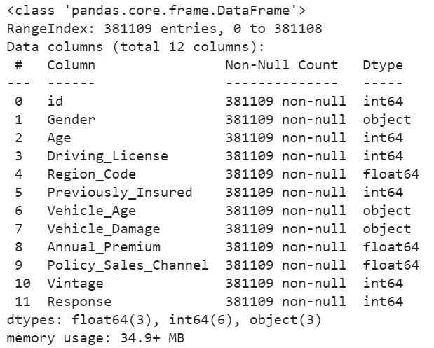
    train_data.info()

    Output:

    end-to-end-output-2

    By looking at the above output, we can say that this data has 9 categorical values, and with this, we can start plotting these values into graphs so that we can get more information out of this data.

    Let’s begin with our target variable.

    By looking at the above output, we can say that this data has 9 categorical values, and with this, we can start plotting these values into graphs so that we can get more information out of this data.

    Let’s begin with our target variable.


    Response valuable

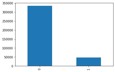
    train_data[‘Response’].value_counts().plot(kind = ‘bar’)

    Output:

    end-to-end-output-3

    Here we can see that we had a huge customer response of 0, which means the majority of customers are not interested in buying vehicle insurance. Now it’s our target to understand how this response variable is dependent on other information given in the data.


    Response with Gender

    train_data[[‘Gender’, ‘Response’]].value_counts().plot(kind = ‘bar’, stacked = True, )


    Looking at this chart, the responses from men are more than women, which is also similar to the positive response.


    Response with Age

    train_data[‘Age’].describe()

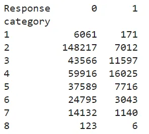
    Here we can see that in the Age column, we have the minimum age of any customer is 20, and the highest age is 85 years. So better visualisation In this section, we are going to separate the age values by the range of 10, and we will be able to see how different age ranges of customers are responding.

    bins = np.arange(1, 10) * 10

    train_data[‘category’] = np.digitize(train_data.Age, bins, right=True)

    counts = train_data.groupby([‘category’,’Response’]).Age.count().unstack()

    print(counts)

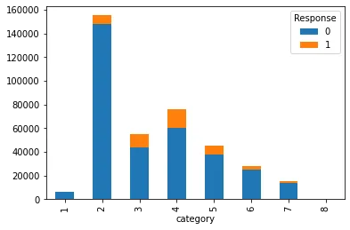
    counts.plot(kind=’bar’, stacked=True)

    end-to-end-7

    end-to-end-7

    Here we can see that most of the records in the data are for the customer age range of 30–40 years, but proportion-wise, customers over 40 years old are more interested in buying vehicle insurance.


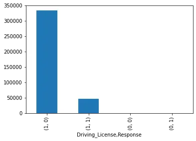
    Response with driving license

    train_data[[‘Driving_License’,’Response’]].value_counts().plot(kind = ‘bar’)

    Output:

    end-to-end-9

    Here we can see that there are few records of customers with no driving license, and they also responded as no, which is fair enough.


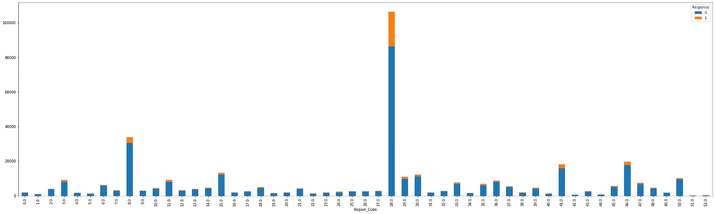
    Response with Region

    counts = train_data.groupby([‘Region_Code’,’Response’]).Gender.count().unstack()

    counts.plot(kind=’bar’, stacked=True, figsize=(35, 10

    Output

    end-to-end-10

    Here we can see the distribution of responses from customers according to the region, and by zooming in, we can see that region 28 holds the most number of records.


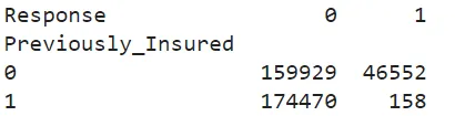
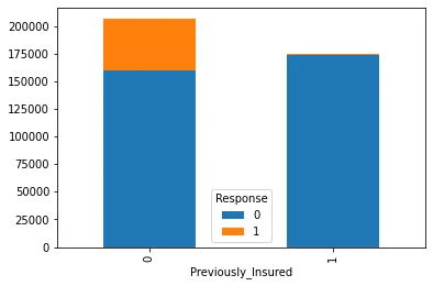
    Previously Insured and Response

    counts = train_data.groupby([‘Previously_Insured’,’Response’]).Gender.count().unstack()

    print(counts)

    counts.plot(kind=’bar’, stacked=True)

    Output:

    end-to-end-11

    end-to-end-12

    Here we can see that most of the positive responses were from customers who had not previously received their vehicle insurance.


    Reponse with Vehicle Age

    With this variable, we can extract information about the most positive responses with respect to vehicle age.

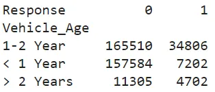
    counts = train_data.groupby([‘Vehicle_Age’,’Response’]).Gender.count().unstack()

    print(counts)

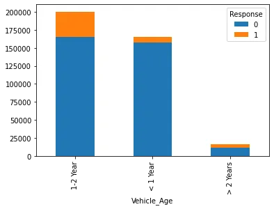
    counts.plot(kind=’bar’, stacked=True)

    end-to-end-13

    end-to-end-14

    With this output, we can assume that the top part of the data is covered by vehicles aged 0 to 2 years, and mostly positive responses are from the customers who have vehicles aged 1 to 2 years.


    Response with Vehicle Damage

    Here we take a look at how customers choose to buy insurance when their vehicle is damaged.

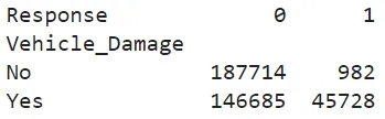
    counts = train_data.groupby([‘Vehicle_Damage’,’Response’]).Gender.count().unstack()

    print(counts)

    counts.plot(kind=’bar’, stacked=True)

    Output

    end-to-end-15

    Here we can see that most customers are ready to buy insurance for their vehicle when it is already damaged.


    Annual Premium

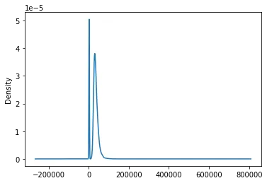
    Since this is a continuous value, we can draw a density plot of the annual premium and see its description to know its minimum, maximum and average value.

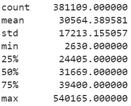
    train_data[‘Annual_Premium’].describe()

    train_data[‘Annual_Premium’].plot(kind = ‘kde’)


    +6

    end-to-end-16

    end-to-end-17

    Here we can see that the minimum size of the annual premium is 2630, and the maximum is 540165, while the average value is around 30564.


    Vintage

    This column represents the count of days of a customer associated with the organisation.

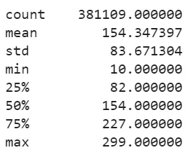
    train_data[‘Vintage’].describe()

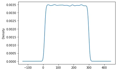
    train_data[‘Vintage’].plot(kind = ‘kde’)

    Output

    end-to-end-8-1

    end-to-end-9-1

    Here we can see that the minimum count of customer association days is 10 days, and the maximum is 299, while the average count is 154 days. So this means most of the customers have been associated with customers for the last 154 days.

    Now that we have completed a basic exploratory data analysis, we will prepare it for the data modelling procedure.


    Data processing

    For modelling the data, we are going to use the scikit learn library that only works with the numerical values, and as we know, we have many string values in the data, so we will need to convert them into numerical data by label encoding we can do.


    Label encoding

    By looking at the data, we know that we have three variables that have categorical values in the form of the string value, so let’s convert these values.

    train_data[‘Gender’]=train_data[‘Gender’].replace({‘Male’:1,’Female’:0})

    train_data[‘Vehicle_Age’]=train_data[‘Vehicle_Age’].replace({‘< 1 Year’:0,’1–2 Year’:1, ‘> 2 Years’:2})

    train_data[‘Vehicle_Damage’]=train_data[‘Vehicle_Damage’].replace({‘Yes’:1,’No’:0})

    train_data.head()

    Output:

    end-to-end-10-1

    Here we can see that all the values are in the numerical format while we have changed binary string values in the form of 0 and 1 binary integer values, and for the vehicle age variable, we have given 0, 1 and 2 as numerical categorical data points.

    Now we would need to split this data into train and test sets so that we can evaluate the fitted model properly.


    Data splitting

    from sklearn.model_selection import train_test_split

    X = train_data.iloc[:, 0:-1]

    y = train_data.iloc[:, -1]

    X_train, X_test, y_train, y_test = train_test_split(X,y, test_size = 0.25, random_state = 4)

    Here we split the data in 75:25 so that we can train a model using 75% of the data and evaluate it with 25% data. Next, let’s move towards the data modelling procedure.


    Data Modelling

    Using the below line of code, we can train a random forest model using our processed data.

    from sklearn.ensemble import RandomForestClassifier

    model = RandomForestClassifier()

    model.fit(X_train,y_train)

    end-to-end-11-1

    Let’s make predictions from the model and plot it once to see whether the model is working well or not.

    y_pred = model.predict(X_test)

    y_prediction = pd.DataFrame(y_pred, columns = [‘predictions’])

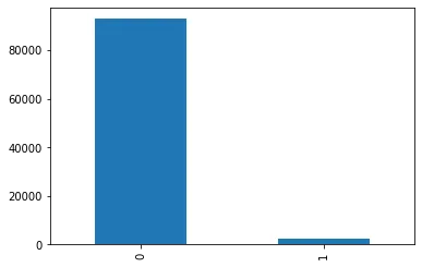
    y_prediction[‘predictions’].value_counts().plot(kind = ‘bar’)

    Ouput:

    end-to-end-12-1

    Here we can see that model is making predictions for both categories. So now, let’s evaluate the model.


    Model Evaluation

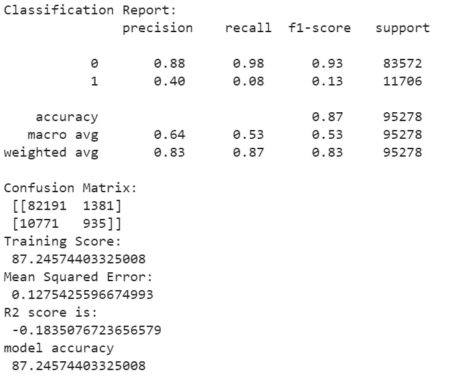
    In the above, we have done the data modelling using the random forest algorithm. Now, we are required to perform a model evaluation to tell about our model’s reliability and performance. Using the below lines of codes, we can measure the performance of our model

    from sklearn.metrics import mean_absolute_error,mean_squared_error,confusion_matrix,r2_score,accuracy_score,classification_report

    print(“Classification Report:n”,classification_report(y_test,y_pred

    print(“Confusion Matrix:n”,confusion_matrix(y_test,y_pred

    print(“Training Score:n”,model.score(X_test,y_test)*100)

    print(“Mean Squared Error:n”,mean_squared_error(y_test,y_pred

    print(“R2 score is:n”,r2_score(y_test,y_pred

    print(‘model parameters n’,model.get_params(

    print(‘model accuracy n’,accuracy_score(y_test,y_pred)*100)

    Ouput:

    end-to-end-13-1

    Here we get most of the metrics in the final report that can be used for model evaluation, and looking at the report, we can say that our model is performing well with such huge data. However, we can make many improvements to the model, which we will discuss later in the article.

    To learn about the evaluation metrics, we can go through this article, where we explain every critical metric we use in real life to evaluate such models.


    To-Do List

    In this procedure, we have performed every basic step which a data modelling procedure needs to go through, and below are the advanced steps we will perform to improve the results of this procedure:

    • More EDA: as we can see in this article, we used only pandas for data visualisation, so in the next article, we will be using more visualisation libraries to perform EDA more properly.
    • SMOTE analysis: in the data visualisation part, we can see that records for a positive response were too low, which can lead to biased modelling, so in the next article, we will see if we can improve the performance using SMOTE analysis.
    • Cross Validation: We know that we got good enough results from the last modelling, and to improve the score, we can also use the cross-validation method so that model can become more reliable.
    • GridSearchCV: it is a method used for finding the optimal model when the model has too many parameters, and Random Forest is one of those models that can be modified by changing parameters.


    References


    About DSW

    Data Science Wizards(DSW ) aim to democratize the power of AI and Data Science to empower customers with insight discovery and informed decision making.

    We working towards nurturing the AI ecosystem with data-driven, open-source technologies and AI solutions and platform to benefit businesses, customers, communities, and stakeholders.

    Through our industry-agnostic flagship platform, UnifyAI, we are working towards creating a holistic approach to data engineering and AI to enable companies to accelerate growth, enhance operational efficiency and help their business leveraging AI capabilities end-to-end.

    Our niche expertise and positioning at the confluence of AI, data science, and open-source technologies helps us to empower customers with seamless and informed decision-making capabilities.

    DSW’s key purpose is to empower enterprises and communities with ease of using AI, making AI accessible for everyone to solve problems through data insights.

    Connect us at contact@datasciencewizards.ai and visit us at www.datasciencewizards.ai

  • What is AI/ML model governance?

    What is AI/ML model governance?

    As every small, medium and large organisation are willing to become data-driven, the application of machine learning and artificial intelligence is increasing rapidly. Also, when we look at the market, we find that AI and ML market is one of the prominent and challenging markets nowadays. However, with these high values, this area also shows us a new source of risk. There can be various reasons, like an inadequately trained data model can lead to bad data-driven decisions, breaking the laws and many more.

    So it becomes a compulsion to define governance in AI/ML development to minimise the risk and improve the development quality. So Let’s look at the broader picture of AI/ML model governance.


    What is model governance?

    When an organisation starts controlling the model development process, usage, and validation or assigns the model’s restrictions, responsibilities and roles, this process can be considered model governance.

    We can compare model governance as a framework where this framework includes a set of strategies that help decide or specify how an organisation manages models within it. These strategies can be of the following type:

    • Strategies to control models in production
    • Strategies for versioning the models.
    • Documentation reaction strategies.
    • Model post-production monitoring
    • Models comply with existing IT policies.

    If any organisation can implement such a framework effectively, then they can get a high level of controllability and visibility into the model’s behaviour in production. At the same time, they get access to operational efficiencies and this help in achieving more benefits from AI investments.

    Increased visibility also allows you to easily identify and resolve the problems and risks of ML and AI, such as models being biased. It also makes us increase the performance of the model in production because enhanced visibility allows you to spot issues that degrade models performance over time, such as data decay, model drift etc.


    Importance of AI/ML Model Governance

    We know that artificial intelligence and machine learning are relatively new areas, and many inefficiencies must be resolved. Model governance not only helps solve many of these problems but also improves every aspect of development and the potential value of any AI project.

    We have already discussed that model governance helps in risk assessment, which is a major importance of AI governance as it ensures that the model stays out of risk with us. Many models are programmed to learn continuously after running them, and they can be biased because of biased data, which affects the decision-making of the model.

    A set of rules in the governance framework allows us to audit and test for the model’s speed, accuracy and drift while in production to prevent further difficulties. Since various clauses can be applied to Ai governance, we can easily find out the ownership and accessibility of the model.

    Such a governance framework can answer the following important questions:

    • Who is the model’s owner?
    • Do relevant rules and regulations restrict a model?
    • Data on which model is trained?
    • What sets of rules and regulations need to comply between the development stages?
    • What are the steps required to monitor models after post-production?

    Who is the model’s owner?

    In an organisation, we can find that various people are arranged to complete various work of any project. So it becomes an important task to keep track of the work of every person involved in the project. This tracking helps improve collaboration, lesser duplication, quality improvement, and improve problem-solving. It always becomes necessary to keep this in the rule book so that well-catalogued inventory can allow people to build on the work together more easily.


    Do relevant rules and regulations restrict a model?

    Often models require following the local or domain rules and laws, such as a recommendation system developed to find relationships between different goods in a supermarket and representing a strong relationship between cigarettes and chewing gum. Most countries don’t allow to advertising of cigarettes, so this kind of business recommendation needs to be dropped. So before deploying a model into production, we should consider the following things:

    • What local government defines regulations and laws relevant to any model’s functionality?
    • What are the ways to test the model’s functionality are complying with defined laws?
    • After making it into production, what will be the ways to monitor the model?

    Data on which model is trained?

    One very important thing about the machine learning model is that their results are indivisibly attached to the training data. So if there is any problem occurs in the development line, it becomes important to find the precise bad data points to replicate the issue. This is an ability in machine learning, and planning based on tracing the issues is crucial to avoid bigger failures.

    Keeping track of the data source is a worthy task because this helps in measuring model drift frequency and stability of the models on old data. So it is always suggested to train the model on a high data range to get different results, but for stability, we should consider a low data range.


    What sets of rules and regulations need to comply between the development stages?

    There are various model development stages involved in the process, and one should have approval at every stage and keep records to ensure a high-quality standard. And it also reduces the chances of failure making their way through the production. This set of rules can tell us about the following things:

    • Data quality
    • Feature engineering
    • Train/Test/Validation or cross-validation
    • Compliance testing
    • Code quality
    • Version control
    • Documentation

    It is highly suggested to get the development thoroughly checked by a qualified team or person outside the development team.


    What are the steps required to monitor models after post-production?

    One of the most important things about model governance is that it gets complete after we become capable of regularly monitoring our deployed model’s performance using various aspects like model drift, data decay and failure in the development pipeline.

    However, these aspects are internally connected, but they all represent their story differently. When things come into the post-production stages, it becomes necessary to maintain the system we have created and the new updates we are trying to give in the system. Early capturing of the likelihood of failure makes the system more accurate and reliable.


    Final words

    In the recent scenario, we have seen that every organisation are willing to become data-driven, or some are already data-driven, where machine learning models are helping them to complete various tasks. To maintain their high performance, effectiveness and quality, it is necessary to care about the model governance, which can lead your model to great success.

    Data Science Wizards (DSW) is an Artificial Intelligence and Data Science start-up that primarily offers platforms, solutions, and services for making use of data as a strategy through AI and data analytics solutions and consulting services to help enterprises in data-driven decisions.

    DSW’s flagship platform UnifyAI is an end-to-end AI-enabled platform for enterprise customers to build, deploy, manage, and publish their AI models. UnifyAI helps you to build your business use case by leveraging AI capabilities and improving analytics outcomes.

    Connect us at contact@datasciencewizards.ai and visit us at www.datasciencewizards.ai

  • How Artificial Intelligence is Advancing the EdTech Industries?

    How Artificial Intelligence is Advancing the EdTech Industries?

    In current scenarios, we all have seen the growth of the EdTech industries. Even after Covid-19, we can say that the growth is doubled. There are many reasons behind this growth; one of them is artificial intelligence has found many gaps to fill. However, the impact of AI is huge across industries. According to Statista, the AI market is expected to reach USD 126 billion by the end of 2025.

    A market and Markets report says that AI in EdTech is expected to grow to 3.68 billion USD by the end of 2023. These statics are sufficient to show EdTech’s reliability on AI. Especially, AI has found various use cases in online education systems. AI enables the industry right from delivering content to assessments and enhancing the learning experience. Here are the top applications of AI using which AI is helping EdTech to get more advanced.


    Customise learning journeys

    We find various unique values regarding learners’ interest and motivation to learn a subject. When we look back at the traditional approach to educational systems, they have been standardised for a long time because it was challenging to make them personalised for individuals. Nowadays, AI approaches have made it easy to create custom-tailored courses of learning based on learners’ behaviour observation and interpretation.

    AI systems can find out the learning gaps based on the performances of learners, as well as these can also find them based on their behaviour in a classroom. As we all know, personalisation has been the KPI of many businesses here, and it plays a significant role in collecting huge audience engagement and focus.

    Because of personalisation, learners get enabled to set up the pace of learning and ensure that they are on the right track of their learning journey.


    Automated Assessments

    Nowadays, we can see the impact of AI on grading because its use can be seen in both quantitative tests (multi-choice questions) and qualitative assessments (essay-based tests). This use of AI saves teachers time on grading and eliminates the chances of divergences based on favouritism and any other kind of corruption.

    In addition, we also get facilitated with understanding the impact and effectiveness of learning programs based on group levels. This analysis can make us stand out from the ground if changes in the curriculum become in the appropriate direction.


    AI Teaching Assistants

    One of the most excellent applications of AI is adaptive chatbots, which can be utilised here as a teacher’s assistant in online programs. Just assume that there is a chatbot that can interact with the learners and clarify many basic doubts. At the same time, they are capable enough to create multiple real-time stages to let learners evaluate their understanding.

    However, human teachers are a great way to teach anything, but they come with a working bandwidth and are incapable of always being available. This causes a gap and also an opportunity for AI to make a bridge. They can be available all the time and give freedom to learners using which they can approach them any time and get clarity.


    Simplifying Non-Teaching tasks

    Here, AI is not only to help the teachers and learners but also comes with many different use cases that are not core to teaching but are very helpful to run institutes easily. For example, using AI, we can easily handle records of students such as attendance, personal information etc., and teachers can be more focused on their teaching work. AI has also shown its capability in enrolment and admission processes so that more forces can get free.


    Final Words

    By looking at the above use cases, we can say the day is not so far where educators will need to rethink the learning journey and impact more students by giving extraordinary learning experiences, retention and focus. Furthermore, with the power of AI systems and tools, the EdTech industries can redefine the future and culture of education, where teachers and learners will be more focused on their actual work instead of being diverted because of too many other constraints or work.


    About DSW

    Data Science Wizards (DSW) is an Artificial Intelligence and Data Science start-up that primarily offers platforms, solutions, and services for making use of data as a strategy through AI and data analytics solutions and consulting services to help enterprises in data-driven decisions.

    DSW’s flagship platform UnifyAI is an end-to-end AI-enabled platform for enterprise customers to build, deploy, manage, and publish their AI models. UnifyAI helps you to build your business use case by leveraging AI capabilities and improving analytics outcomes.

    Connect us at contact@datasciencewizards.ai and visit us at www.datasciencewizards.ai

  • A Simple Introduction to Ensemble Learning

    A Simple Introduction to Ensemble Learning

    In one of our last articles, we discussed that random forest is an ensemble machine learning algorithm that predicts based on the combined predictions of multiple decision tree models. Since we found that ensembling multiple models or being an ensemble learning model is the main reason behind the success rate of any random forest model, this generates a curiosity to know more about the ensemble learning topic. So in this article, we will discuss the theoretical details of the ensemble machine learning method. We will cover the following important points about it:


    Table of content

    1. What is Ensemble Machine Learning
    2. Ensemble learning Techniques

    Simple Techniques

    1. Max Voting
    2. Averaging
    3. Weighted Averaging
    4. Advanced Techniques
    5. Stacking
    6. Blending
    7. Bagging
    8. Boosting

    What is Ensemble Machine Learning?

    As discussed above, ensemble learning is an approach that comes under supervised machine learning, where we use the combined results of several supervised learning models. So let’s try to understand it more using an example. Let’s say a person has written an article on an interesting topic, and he wants to know the preliminary feedback before publishing it. So he thinks about the following possible ways.

    • Ask a friend to rate the article: In this way, there is a huge possibility that a friend of his gave a nice rating for a horrible work because he didn’t want to break the heart of his friend.
    • Ask five friends to rate the article: This way, he got the proper idea of the article because some of them chose to give an honest rating to him. But there is also a possibility that the people are not subject matter experts on the topic of his article.
    • Ask 50 people to rate the article: Here, he has included all his friends and some strangers to give feedback and got more generalized and diversified feedback. This approach can be the best of all the approaches he chose to get feedback for his work.

    Here we can infer that if the person uses a diverse group of people to get the feedback, he will get better results as compared to a nondiverse group or individuals. This way can also be applied in machine learning, where a set of multiple models can give better results than a single model. This diversification in machine learning can be achieved using ensemble learning models.

    Here we got a basic understanding of the ensemble learning technique. Let’s take a look at the various techniques using which we can perform ensemble learning.


    Ensemble Learning Techniques

    The following are techniques to perform ensemble learning:

    Simple techniques

    • Max Voting: we generally use this method for solving classification problems. Using each data point, multiple models give their outcome, and this outcome is considered as the vote. Using the majority vote-winning technique, we reach the final result.

    Suppose there in the above example, the person chose to follow the second way and asked five friends to give feedback. If 4 or 3 out of 5 are on the positive side, which means they give more than 2 rating points, then the person will make the article published. The result of this structure of ensemble learning will take like as follows:

    • Friend 1 = 3
    • Friend 2 = 4
    • Friend 3 = 5
    • Friend 4 = 2
    • Friend 5 = 3
    • Averaging: Just like in the max voting system, here also, all the models take each data point to make predictions, but we consider the final result as the average of results from all the models. The averaging method is mostly applied in regression problems.

    By the above-given results, we can calculate the final result in the following way:

    (3 + 4 + 5 + 2 + 3)/5 = 3.4

    • Weighted Average: This technique of ensemble learning is different from the other methods because we use the importance of each model as the weight, and the final result comes out from the weighted average method.

    Let’s say 2 out of 5 friends are given more importance in the above example, and because of this weight or importance, the final result will be as follows.

    (3 + 4 + 5 + 2 + 3)/5 = 3.4

    Advanced techniques

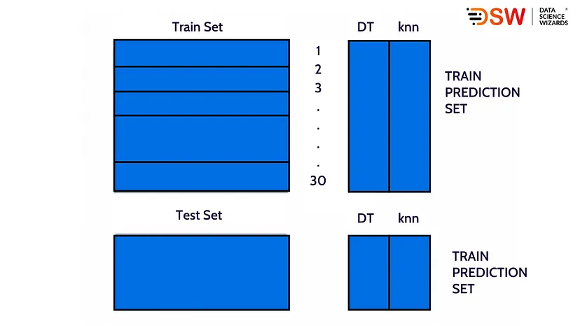
    • Stacking: if the above-discussed methods can be considered basic ensemble learning methods, then methods after this can be considered advanced ensemble learning. Stacking is a method where several learners are attached one after another. Decision tree, KNN and SVM algorithms can be considered examples of base models used in stacking learning. The following steps a stacked ensemble learning model takes to give final results:
    1. Splits the training set into n parts.
    A-simple-1

    1. A base model learns from the nine parts and predicts the 10th part of the data.
    A-simple-2

    1. The base model gets fitted on all parts of the training data.
    2. Using the trained model, we calculate the predictions using the test data.
    A-simple-3

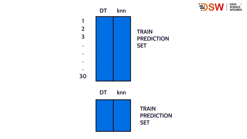
    1. Steps 2, 3 and 4 are repeated using different models like KNN or SVM, and that also gives predictions but different from the first cycle.
    A-simple-4

    1. Predictions based on train data are considered as the feature to build a new model.
    A-simple-5

    1. The final or new model gives the final prediction based on the test set.
    • Blending: Blending is almost similar to the stacking approach, but the use of validation data makes it different, unlike the stacking method. It gives the predictions from the validation set only. This validation set and prediction were made using the validation set used to run on the test set. The steps this method uses are as follows:
    1. The whole data is split into three sunsets: train, test and validation.
    2. Models are trained on the training set.
    3. A validation set and a train set are used to make the prediction.
    4. Validation set and predictions made using validation set used as a feature to train a new model.
    5. A new model and test data are used to make the final prediction.
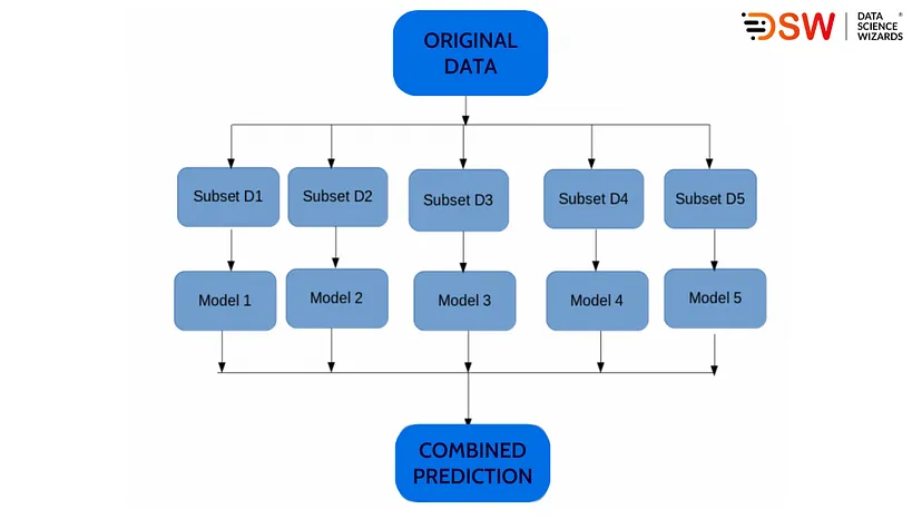
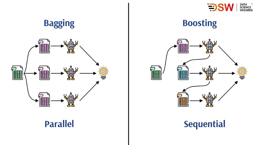
    • Bagging: Bagging is an advanced form of ensemble learning where it uses multiple models to give their individual results on a sub-part of data. By combining these results gives a final outcome. Since multiple models have a high chance of giving the same results while inputs are similar, bootstrapping comes into the picture to fail this condition. It helps create various subsets of whole data and then trains multiple models on those subsets. The below picture is an illustration of the bagging technique.
    A-simple-6

    The following steps this technique uses to learn from the data:

    1. Subsets are created from the original data.
    2. A base model is assigned to learn from each subset.
    3. The final prediction comes out as the combined result from all the models.
    • Boosting: Boosting ensemble learning can be considered a sequential learning method, where each subsequent model tries to correct the errors from the previous model. It means that the outcomes of a succeeding model depend on the outcome of the previous model. The following steps this technique takes to complete the modelling:
    1. Creation of a subset from the main data.
    2. At the initial stages, all the data points have similar weightage.
    3. A base model gets trained on the subset and gives predictions using the whole data.
    4. Errors are calculated using the initial model’s original value and predicted value.
    5. Incorrectly predicted data points take higher weights.
    6. Again a base model is used to get trained and give predictions on the dataset.
    7. The process from steps 3 to 6 is repeated until the final learner doesn’t occur.

    Final words

    Here in the article, we have discussed the basic introduction of ensemble machine learning. Using an example, we tried to understand how it works and learn about the different ensemble learning techniques, such as max voting, averaging, bagging and boosting. In our next articles, we will discuss the models based on ensemble learning techniques.


    About DSW

    Data Science Wizards (DSW) is an Artificial Intelligence and Data Science start-up that primarily offers platforms, solutions, and services for making use of data as a strategy through AI and data analytics solutions and consulting services to help enterprises in data-driven decisions.

    DSW’s flagship platform UnifyAI is an end-to-end AI-enabled platform for enterprise customers to build, deploy, manage, and publish their AI models. UnifyAI helps you to build your business use case by leveraging AI capabilities and improving analytics outcomes.

    Connect us at contact@datasciencewizards.ai and visit us at www.datasciencewizards.ai

  • Getting Started with Machine Learning Algorithms: Random Forest

    Getting Started with Machine Learning Algorithms: Random Forest

    In supervised machine learning, there is a plethora of machine learning models like linear regression, logistic regression, decision tree and others. we use these models to resolve classification or regression problems, and ensemble learning is a part of supervised learning that gives us models that are built using several base models. Random forest is one of those ensemble learning models that are popular in the data science field for its high performance.

    Technically, random forest models are built on top of decision trees and we have already covered the basics of a decision tree in one of our articles, so we recommend reading the article once to understand this article’s topic clearly. In this article, we will talk about random forests using the following points.


    Table of content

    • What is Random Forest?
    • How Does a Random Forest Work?
    • Important Features
    • Important Hyperparameters
    • Code Example
    • Pros and Cons of Random Forest

    What is Random Forest?

    Random forest is a supervised machine-learning algorithm that comes under the ensemble learning technique. In supervised machine learning, a random forest can be used to resolve both classification and regression problems.

    As discussed above that, it comes under the ensemble learning technique, so it works on top of many decision trees. We can say that decision trees are the base model of a random forest. The algorithm simply builds many decision trees on different data samples, and using the majority vote system solves the classification problem. In the case of regression, it uses the average of the decision trees.


    How does a Random Forest Work?

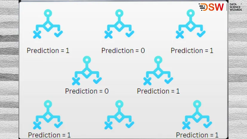
    When we talk about the working of the random forest, we can say that it gives outcomes by ensembling the results of many decision trees. Here if we talk about a classification problem, each decision tree predicts an outcome and whatever the class gets majority votes comes out as the final result of a random forest. Let’s take a look at the below image.

    rf-1

    When we talk about the working of the random forest, we can say that it gives outcomes by ensembling the results of many decision trees. Here if we talk about a classification problem, each decision tree predicts an outcome and whatever the class gets majority votes comes out as the final result of a random forest. Let’s take a look at the below image.

    The above image also gives the intuition behind the ensemble learning technique, where the final prediction is made by combining the results of several other models. The ensemble learning technique can be followed using two ways:

    1. Bagging: this way, we divide data into various subsets and train the base models like decision trees in a random forest, and the majority vote for any class comes out as the final result.
    2. Boosting: this way, we combine weak learners with strong learners and make a sequence of the model so that the final model is most accurate amongst every learner. For example, XG boost and ADA Boost models.
    rf-2

    Random forest in ensemble learning uses the bagging method. We can say that every decision tree under the random forest uses a few samples from the whole training data to get trained and give predictions. Let’s talk about the steps involved in training the random forest algorithm.


    Steps involved

    1. First, it extracts n number of subsets from the dataset with k number of data points that we call n subsets.
    2. n number of decision trees are constructed to get trained using n subsets.
    3. Each decision tree gives predictions.
    4. Final predictions are generated using the majority voting system for the classification problem and an averaging system for the regression problem.

    Using the above four steps working of a random forest gets completed. Next, let’s discuss the important features of a random forest.


    Important features

    1. Highly immune to dimensionality: Since all data features are not considered in the making of decision trees, the whole random forest gives high performance even in a situation where data is high-dimensional.
    2. Diversity: every decision tree uses some of the features from the data. That’s why the training procedure becomes different for the different decision trees. At final, we get more optimum results.
    3. Data split: while making a random forest, we don’t really need to spit data in train and test because there will always be some percentage of data unknown for a decision tree.
    4. Stable: random forests are stable algorithms when modelled because the majority voting or averaging system is used to make the final prediction.
    5. Parallelization: as we know, every individual decision tree uses a part of the main data. It makes full use of the CPU to train random forests.
    6. No overfitting: as the final results from the random forest come from the majority voting or averaging system and the decision tree uses subsets to get trained, there are fewer chances of overfitting.

    Important Hyperparameters

    In the above we have discussed the working and features of random forests, here we will discuss the important hyperparameters of any random forest using which we can control the random forest while increasing its performance and making it’s working or calculation faster.

    1. n_estimators- The number of decision trees required to build the random forest.
    2. max_features- Maximum number of features that random forest will use from data to split the data.
    3. mini_sample_leaf — minimum number of leaves is required to split the decision tree node.
    4. n_jobs — we use it to speed up the calculation of random forest because it tells the number of processors a system needs to train the model.
    5. random_state- just like for other models, it controls the randomness of the sample.

    Code Example

    In the above discussion, we have seen how random forest work and their important hyperparameters. Now after knowing this, we need to know how it works using any tool. So here we will look at the simple implementation of the random forest using the python programming language.

    We will use randomly generated data and the sklearn library in this implementation. So let’s start with generating data.

    from sklearn.datasets import make_classification
    X,y = make_classification(n_samples = 2000, n_features = 6, n_informative = 3)
    print(‘data features n’,X)
    print(‘data_classes n’, y)

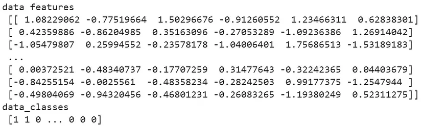
    Output:

    rf-3

    Here we can see features and classes of randomly generated data. In the making of data, we have generated 2000 samples that have 6 features and one target variable.

    Let’s build a model

    from sklearn.ensemble import RandomForestClassifier
    clf = RandomForestClassifier(max_depth = 4, random_state = 42)

    Here we have created an object named clf that consists of a random forest classifier. Let’s train the model.

    clf.fit(X,y)
    print(‘count of the decision trees :’,len(clf.estimators_

    Output:

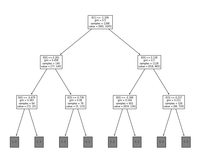
    Here we can see that 100 decision trees are under the random forest. Now we can draw a decision tree from our random forest using the following lines of code:

    import matplotlib.pyplot as plt

    from sklearn import tree

    plt.figure(figsize=(12, 10

    tree.plot_tree(clf.estimators_[0],max_depth = 2)

    plt.show()

    Output:

    rf-5

    Here we have implemented a random forest, and to increase the explainability, Now we can draw a decision tree from a random forest using the following lines of code:

    print(clf.predict([[0, 0, 0, 0, 0, 0]]

    print(clf.predict([[1, 0, 1, 0, 1, 1]]


    Output:

    rf-6

    Now results from the model are in front of us and this is how we can implement a basic random forest. Let’s take a look at the pros and cons of the random forest algorithm.


    Pros and Cons of Random Forest

    Pros

    1. We can use it for both classification and regression problems.
    2. It does not overfit.
    3. It can also work with data that contains null values.
    4. High-performing with high dimensional data.
    5. It maintains diversity in the results.
    6. Highly stable.

    Cons

    1. Random forest is a highly complex algorithm.
    2. Training time is more because it takes more time to calculate, develop and train decision trees.

    Final words

    Under the series of articles, this article consisted the information about the random forest, which is a machine learning algorithm used to resolve problems that come under supervised learning. In the article, we have discussed the what, why and how of random forests. Using an example we looked at its implementation. Looking at the pros and cons of this model, we can say that it has such features and functionality that gives us higher accuracy. Still, before using this model we should understand the basic concept behind the model so that we can tune it appropriately.


    About DSW

    Data Science Wizards (DSW) is an Artificial Intelligence and Data Science start-up that primarily offers platforms, solutions, and services for making use of data as a strategy through AI and data analytics solutions and consulting services to help enterprises in data-driven decisions.

    DSW’s flagship platform UnifyAI is an end-to-end AI-enabled platform for enterprise customers to build, deploy, manage, and publish their AI models. UnifyAI helps you to build your business use case by leveraging AI capabilities and improving analytics outcomes.

    Connect us at contact@datasciencewizards.ai and visit us at www.datasciencewizards.ai

  • Evaluation Metrics for Machine Learning or Data Models

    Evaluation Metrics for Machine Learning or Data Models

    In data modelling, after a point, it becomes easy to train a model using historical data. Still, because of the different characteristics of models and datasets, it becomes difficult to evaluate the model using the right set of evaluation metrics. The model evaluation process goes through understanding the model and data to understand the right evaluation metrics for a problem. Before applying any evaluation metric in the process, we should be knowledgeable about important metrics to evaluate the model correctly. So in this article, we will cover the basics of different evaluation metrics. The list of these evaluation metrics is as follows:


    Table of contents

    • Confusion Matrix
    • Classification Accuracy
    • Precision/Specificity
    • Recall
    • F-1 Score
    • AUC-ROC
    • Root Mean Square Error(RMSE)
    • Cross-entropy Loss
    • Gini Coefficient
    • Jaccard Score

    Confusion Matrix

    It is a matrix of size (a x a) where ‘a’ is the number of classes available in the classification data. The x-axis of this matrix can consist of the actual values and the y-axis can consist of the predicted values or vice versa. If the dataset has only two classes or belongs to the binary classification problem then the size of the matrix will be 2 X 2.

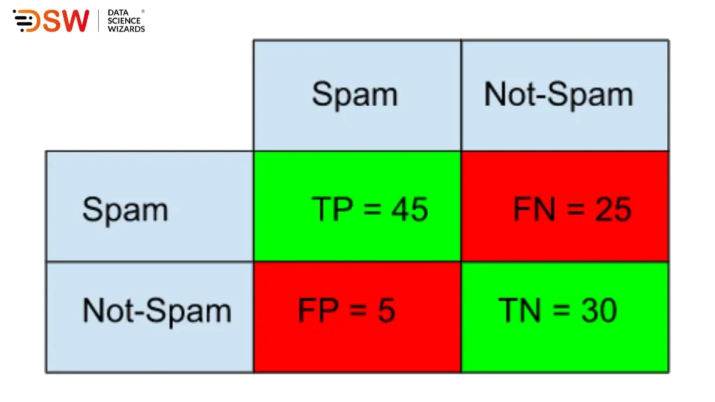
    We can also call it an error matrix which is a matrix representation of model performance comparing the predictions of the model to ground truth labels. The below image is an example of a confusion matrix for model classifying between Spam and Not Spam.

    cm-1

    Here is the following interpretation we can do with the confusion matrix:

    • True Positive(TP): Correct Positive Predictions
    • True Negative(TN): Correct Negative Predictions
    • False Positive(FP): Incorrect Positive Predictions
    • False Negative(FN): Incorrect Negative Predictions

    Using the above values, we can calculate the following rates:

    • True Positive Rate(TPR) = TP/Actual Positive = TP/ (TP + FN) = 45/(45+25) = 0.65
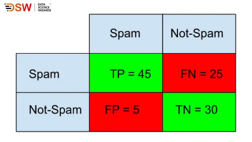
    • False Negative Rate(FNR) = FN/Actual Positive = FN/ (TP + FN) = 25/(45+25) = 0.36
    • True Negative rate = TN/Actual Negative = TN/ (TN + FP) = 30/(30+5) = 0.85
    • False positive rate = FP/Actual Negative = FP/ (TN + FP) =5/(30+5) = 0.15

    Here using the values in the above confusion matrix we have calculated 4 evaluation metrics.


    Classification Accuracy

    Using the above interpretation, we can easily calculate the classification accuracy using the following formula:

    Classification accuracy = (correct prediction) / (all prediction) =(TP + TN) / (TP + TN + FP + FN)

    ca-2-1

    According to the above confusion matrix, classification accuracy will be

    Classification accuracy = (45 + 30)/ (45 + 30 + 5 + 25) = 0.71

    Here we can see the accuracy of the model is 0.71 or 71%. This means that model will give 71 right answers out of 100 questions.


    Precision/Specificity

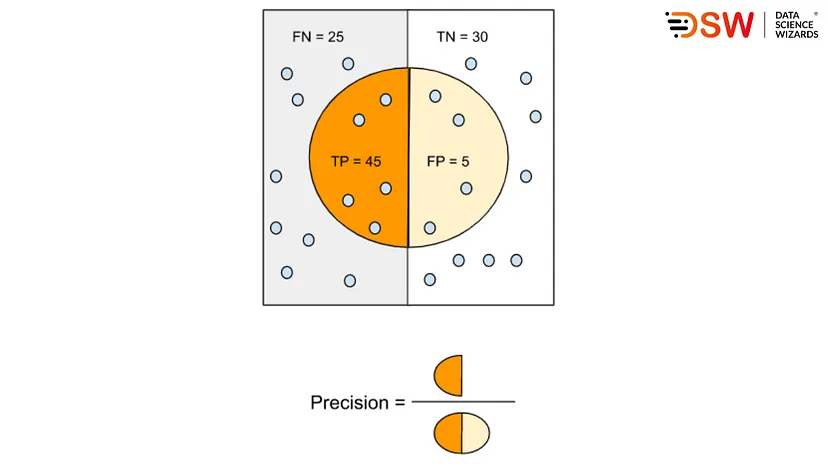
    With imbalanced data, classification accuracy is not the best indication to represent the model performance. In such conditions, we need to deal with a class-specific problem and precision or specificity is the best way to check the model’s performance. To get the value of this indicator, we need to have the true positive divided by the sum value to false positive and true positive.

    Precision/Specificity = True Positive(TP) / (True Positive(TP) + False Positive(FP))

    By this calculation, we quantify the predictions from the model that actually belongs to the positive class. Let’s have a look at the below diagram:

    precision-3-1

    Recall

    The recall is a metric that represents the quantification of correct positive predictions that are made out of all positive predictions. Unlike precision, metrics recall comments on only the correct positive predictions made out of all positive predictions so that an indication of missed positive predictions can be provided. The below formula can be used to calculate the recall of any model:

    Recall = True Positive(TP) / (True Positive(TP) + False Negative(FN))

    Let’s take a look at the below diagram:

    recall

    According to the above diagram, the recall will be:

    Recall = 45/(45 + 25) = 0.64

    This means 64% time relevant items are retrieved.


    F-1 Score

    We can calculate the F1 score using precision and recall, which can be considered an excellent metric to use when the data is imbalanced.

    F1 Score = 2*(Precision *Recall) / (Precision + Recall)

    Using the above precision and recall we can calculate the F1 score in the following way:

    F1 score = 2 * (0.90 * 0.64)/(0.90 + 0.64) = 0.75

    We can consider this metric as the harmonic mean of precision and recall. That’s why this gives equal importance to precision and recall metrics. This metric can also be manipulated by adding in the equation so that more weight to one of them can be given. For example

    F = (1 + 2)* (Precision * Recall)/ (Precision*2) + Recall


    AUC-ROC

    AUC-ROC (Area Under the Curve-Receiver Operator Characteristic) is a curve that makes a plot between TPR and FPR at different threshold values while separating the signals from the noise. The area Under the Curve represents the ability of the model to predict between classes, and the plot uses it as the summary of the ROC curve.

    The AUC varies between 0 and 1, and as the AUC increases, the classifier’s performance improves. If the AUC is one, then we can think of a classifier that is highly capable of distinguishing between all the Positive and the Negative classes correctly.


    Root Mean Square Error(RMSE)

    This metric is used to measure the performance of a regression model, which assumes the errors are normally distributed and unbiased. This is the standard deviation of the prediction errors. Prediction errors are a measure of the distance of the data points to the prediction line. Using the below formula, we can calculate it:

    RMSE = i = 1N(Prediction — Actual)2/N

    Using the below image we can understand what is the prediction errors.


    Cross-entropy Loss

    It is also known as Log Loss and is famous for evaluating neural networks’ performance because it helps overcome the vanishing gradient problems. By summing the log value of prediction probability distribution for incorrect predictions, we can calculate the Cross-entropy Loss.

    Hp(q) = -1/n(i=1Nyi.log(p(yi))+(1-yi).log(1-p(yi)))

    To evaluate the model using these metrics we usually make a graph between log loss and predicted probability as given in the below image:


    Gini Coefficient

    This can be calculated using the AUC-ROC number, this is a ratio of ROC and diagonal line. If the value of this coefficient is more than 60%, then model performance is good, and one thing which is important here is that we use it only with classification models.

    Gini = 2*AUC — 1


    Jaccard Score

    This score represents the similarity index between two datasets. Similar to RMSE, it gives a value between 0 and 1, where 1 represents closer similarity. To calculate this, we need to divide the total number of data points in both sets by the number of observations in either set.

    J(A, B) = |A∩B| / |A∪B|


    Final words

    Here in the above, we have discussed some of the important metrics we use to evaluate the data models in real life. Since models and datasets have different conditions and characteristics, we can optimise different performance levels. So the model performance evaluation needs to be done rightly by knowing the characteristics of different evaluation metrics.

  • How Artificial Intelligence is Advancing the Gaming Industry

    How Artificial Intelligence is Advancing the Gaming Industry

    The gaming industry is one of those industries that is chock full of technology and future probabilities. The reason is the component, platforms and objectives of a single game include various components made using technology and logic. With this amount of technology implementation in the industry, we can easily say that it is a compulsion for these technologies to include AI with them. The primary purpose of applying AI in gaming is to make the games more responsive and provide flexible game experiences to users.

    The reality is that AI is what makes video or computer games more challenging and brings life to virtual games. In simple words, nowadays, AI environments are incorporating both virtual and augmented reality so that the future of gaming can become more robust and efficient. There are various possibilities in the industry where AI, machine learning and data science can take part to develop more. Some of them are discussed below:


    AI in Development and Programming

    gaming-1

    As we all know, a fundamental requirement of Implementing AI in any industry is data. For example, in the gaming industry, AI uses data to create an existence where characters and bots can survive by performing basic actions. These collected data also help AI to create environments including situations, objects and objectives.

    The above-given application represents how AI helps in game development, but when it comes to programming, the feature and levels of game AI play a crucial role. Gaming AI can optimise the skills and emotions of the players and tailor the game accordingly. AI-enabled games are also capable of identifying the player’s intent. This is how AI assists games to become more challenging.


    Providing skills to NPCs

    gaming-2

    In games, NPCs (Non-Player characters) are known as the most difficult part of the game to design. To make the game more challenging, NPCs need to be stronger, and here, AI finds a way of being involved in the gaming industry. AI makes NPCs intelligent game characters which can act as tough as any human players control them. By determining the behaviour of these characters, AI empowers them with actions. Usually, decision trees and random forest algorithms are used to determine the behaviour of these characters.


    Users Journeys

    gaming-3

    Leveraging the gaming designs and elements in a business operation is called gamification of the business. This process aims to make habit-forming commodities that can empower us with large-term retention and engagement. Placing AI in such development can make the process more efficient by classifying human behaviour and responses. A positive user experience can lead to increased engagement and business.


    Realistic Gaming

    gaming-4

    Virtual reality and augmented reality are technologies that are AI-enabled and have been growing as the involvement of Ai in the industry has increased. Such tools and technologies help developers create intelligent, appealing games. Nowadays, games have become easily understood, making their use easy and captive, thanks to AI that helps developers understand the scope and gamers to understand the game. AI helps developers to make a game that can explain and react to users’ activities, whereas in gaming time, predict the next move so that game can act accordingly.


    Smarter games

    Conversational AI is playing a significant role in advancements of the gaming industry, and many gamers can witness that using this support of AI games is providing A wide range of support to its users. Even nowadays, we can see that these AI bots are available in the gaming console.

    Using AI, developers can aim to create a strong framework inside the games. Recent AI technologies like Receiving Recognition And Reinforcement Of Design help characters of the games to learn from their behaviour and develop accordingly.


    Smarter Mobile Games

    gaming-5

    There is no doubt that mobile phones nowadays are strong devices, and some are built to play mobile games. This sector of the gaming industry has shown rapid growth in recent years. With the help of artificial intelligence, developers are making mobile games smarter than before. PUB-G mobile is one of the simple examples where we can witness the trend of mobile game development. Not only visually but also various other features look like they developed a lot in the game, many of which result from AI and machine learning.


    Final words

    Looking at the above points, we can conclude that artificial intelligence will impact video and mobile gaming. As the data and information become accessible and straightforward for game developers, there will be a possibility of further developments in the game visuals and characters that can create their own story.

    In future, we can see AI-based player profiles in the game structure to give users a more challenging gaming environment so that the field can become more realistic and be considered a sport instead of just a field for passing the time. AI is also providing facilities for developers to showcase their full potential.


    About DSW

    Data Science Wizards (DSW) is an Artificial Intelligence and Data Science start-up that primarily offers platforms, solutions, and services for making use of data as a strategy through AI and data analytics solutions and consulting services to help enterprises in data-driven decisions.

    DSW’s flagship platform UnifyAI is an end-to-end AI-enabled platform for enterprise customers to build, deploy, manage, and publish their AI models. UnifyAI helps you to build your business use case by leveraging AI capabilities and improving analytics outcomes.

    Connect us at contact@datasciencewizards.ai and visit us at www.datasciencewizards.ai

  • 5 Basic Types of Databases

    5 Basic Types of Databases

    We have all witnessed the trend of generating data in current scenarios. There is no doubt that it is increasing daily whether the generated data is relevant or irrelevant. And this reveals the massive necessity of smartly designed databases so that massive chunks of data can be handled and proceed accurately.

    As we know, databases are the first starting point of any data process. It becomes a compulsion for us to understand which data we have, what process is required to complete and, based on many constraints, what kind of databases we can use. As deep we go into the topic, it becomes more complicated. It is highly suggested to get started with this subject, one should begin by knowing the basic types of databases, so using this article, we are going to discuss the following basic types of databases:

    • Hierarchical Database
    • Network Databases
    • Object-Oriented Database
    • Relational Database
    • Non-relational Database

    Let’s start with our first Database

    1. Hierarchical Database

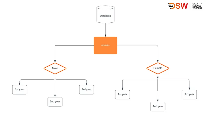
    Like other hierarchical programs, this database stores the data categorised in ranks and levels. To do so, we categorise data using a common point linkage. For example, in gender classification data, humans are a common link between males and females. As given in the below diagram:

    db-1

    The above diagram shows that the database data is structured in a hierarchy where humans are classified by gender. After that, genders are organised based on year. For gender, human is the common link, and for the year of study, male and female as their common link.

    By looking at the structure of stored data, data is organised using the parent-child relationship. As the multiple data element will be added to their parent node, it would resemble a tree structure. We can say that because of this structure, we can not easily mine such databases. Also, with the addition of data in such a structure, we need to do lengthy traversal through the database.


    2. Network Databases

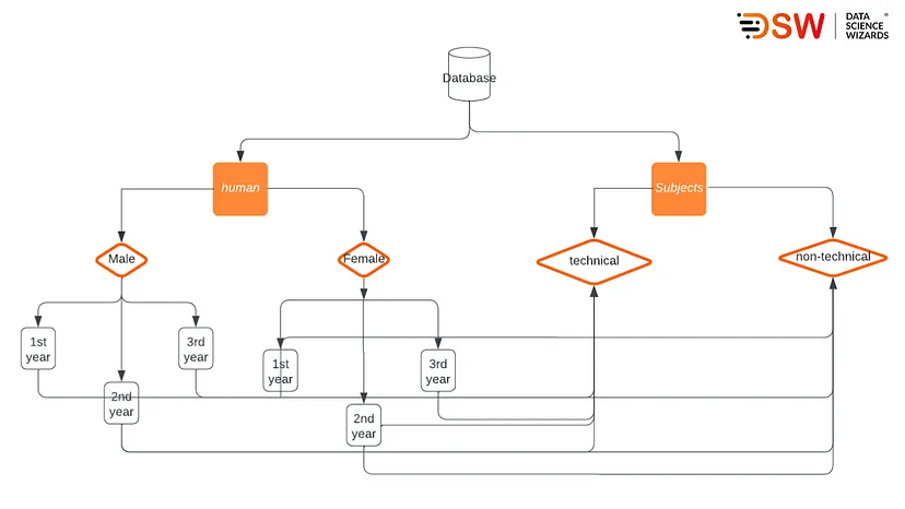
    We can think of this type of database as a hierarchical database, but here the child nodes are allowed to link with more than one parent node. With such linkage options, we find a network-like structure of databases and files linked with multiple threads. For example, let’s take a look at the below diagram:

    db-2

    The above diagram shows that it is a complex structure, but they are more capable of representing two or more directional relationships. The major disadvantage of this type of database is they are difficult to alter and highly structurally dependent.


    3. Object-Oriented Database

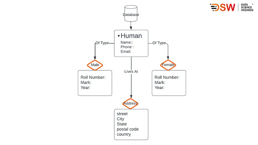
    An object-oriented database (OOD) is a database system that can store and work with complex data objects. In layman’s terminology, it is a way of storing data organised around objects rather than actions. The data stored in such a database can be represented as an object that responds to a database model’s instance. This architecture lets us reference and calls objects easily. For a better understanding, Look at the below diagram:

    db-3

    In the above charts, we can see how the different information of data is linked to each other using a method or command. Using such architecture, we can easily find the gender of any person using the “of type” method and his/her address using the “lives at” method. The main objective behind architecting such a database is to reduce the workload on the database.


    4. Relational Database

    As the name suggests, his type of database stores every piece of information related to every piece of information. It is one of the widely used types of database because it often works n the production line with its management system. Every piece of information stored in this database has a unique identity which we usually call the records.

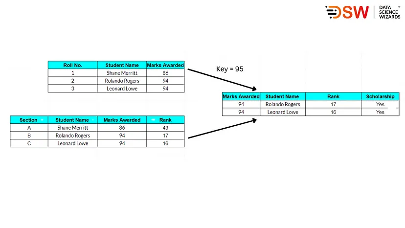
    The unique identification of every piece of information is that it stores the data in tabular form. Primary keys are the linkage between every row of tables, and foreign keys are the linkage between the tables.

    db-4

    We can use the above diagram to understand the concept of keys in a relational database. Its capability of storing data in tabular form it has exceedingly popular. Simple languages developed for this type of database make interaction with the database simple.


    5. Non-relational Database

    These types of databases are the most basic types of data storage systems as they give the simplest way to store and retrieve data. In addition, these databases include simple design, finer controllability and simple scaling to different machines. The above-discussed databases use relational data, but here data structure inside a non-relational database is different so that it can make some options faster.

    There are several advantages of using non-relational databases, such as high scalability and high availability, while being open source, complex backup, and large document sizes are some of the disadvantages of this database. MongoDB and Cassandra are examples of Non-Relational databases.


    Final words

    Here we have ear the basic knowledge about the five basic types of databases, where many work based on the relationship between data values, many works based on the relation between tables, and many can help store both relational and non-relational data values. However, in real-life scenarios, we often find that industries tend to focus on implementing databases based on their requirements. So it becomes a compulsion for us to keep track of the basic knowledge of databases, which we tried to cover in this article.


    About DSW

    Data Science Wizards (DSW) is an Artificial Intelligence and Data Science start-up that primarily offers platforms, solutions, and services for making use of data as a strategy through AI and data analytics solutions and consulting services to help enterprises in data-driven decisions.

    DSW’s flagship platform UnifyAI is an end-to-end AI-enabled platform for enterprise customers to build, deploy, manage, and publish their AI models. UnifyAI helps you to build your business use case by leveraging AI capabilities and improving analytics outcomes.

    Connect us at contact@datasciencewizards.ai and visit us at www.datasciencewizards.ai

  • Assumptions, and the Pros & Cons of Data Models

    Assumptions, and the Pros & Cons of Data Models

    In every sector of life, before applying anything big or small we may need to consider some of the assumptions and know the pros and cons. Similarly, when we talk about data science and data modelling we have a variety of options that can help resolve data-related problems and make data-driven decisions. The main problem that comes to our mind is on choosing one of those options. Where A well-trained model can give fruitful results, a wrong-fitted model can exploit the whole scenario. So using this article, we can get some critical information about Assumptions, and the pros and cons of data models that are really usable in a real-life scenario. During the course we will read about the following model:

    • KNN (K-Nearest Neighbour)
    • Logistic Regression
    • Linear Regression
    • Support Vector Machine
    • Decision Trees
    • Naive Bayes
    • Random Forest
    • XGBoost

    KNN (K-Nearest Neighbour)

    Assumptions:

    • Distance metrics like Manhattan and euclidean can be used to measure the distance of data in feature space.
    • Every training data point should involve a set of vectors, and class names should be concerned with every training data point.
    • If only two classes are in the dataset, then the value of K should be an odd number.

    Pros:

    • A white box algorithm means the mechanism is easy to implement and interpret.
    • Due to the lack of parameters, this algorithm does not requires assumptions to be strictly followed.
    • Using this algorithm, we can push training data at runtime, make predictions simultaneously, and make the procedure faster than other algorithms. This means a particular training program or step is not required.
    • The training step is not required, so the new data points addition step becomes easy.

    Cons:

    • With large and sparse data set algorithm becomes inefficient and slow because of the cost of distance calculation between data points.
    • Sensitive when data includes outliers inside.
    • If missing values or null values are available, then it can not work.
    • Calculations such as feature scaling and normalization are required in addition to distance calculation.

    Logistic Regression

    • As minimal as possible or no multicollinearity is required in the independent data variables.
    • Independence between data variables is needed.
    • With Large datasets, this algorithm performs much better.

    Pros:

    • With less computational power, it is also a white-box algorithm.
    • Fewer assumptions are required in terms of class distribution.
    • Less calculation is required to classify unknown data points.
    • Highly efficient when features are linearly separable.

    Cons:

    • This algorithm uses a linear decision surface to classify data, so it becomes problematic when there are non-linear problems.
    • Its working is dependent on the probabilistic approach that causes overfitting in high dimensional data space.
    • Weak in obtaining complex relationships.
    • Large data of all categories are required for training.

    Linear Regression

    Assumption:

    • There should be linearity between data points.
    • Similar to logistic regression, As minimal as possible or no multicollinearity is required in the independent data variables.
    • The variance in error terms or residuals should be the same for any value of the target variable.

    Pros:

    • Highly efficient when independent and dependent variables are linearly related.
    • Regularization techniques can be applied when the model is overfitted.

    Cons:

    • Data should be linearly separable.
    • Model performance weakens when outliers are in the data.
    • Data independence is difficult to obtain.

    Support Vector Machine

    Assumption:

    • Identical distribution and independence in data are required.

    Pros:

    • Highly efficient with high-dimensional data even when the number of samples is lower than the number of dimensions.
    • Memory efficient.

    Cons:

    • The high-level calculation makes the algorithm slower.
    • Low interpretability.
    • Low efficiency when the dataset is noisy.
    • Good with high dimensional data, but the large sample size makes it inefficient.

    Decision Trees

    Assumptions:

    • At the start of training, the whole data need to think as training data.
    • Data should be distributed recursively based on the attribute value.

    Pros:

    • Less data preparation is required.
    • Calculations like data normalization and scaling are not required.
    • Higher interpretability can be explained using if-else conditions.
    • a Low number of missing values doesn’t affect the results.

    Cons:

    • The higher calculation requires a lot of time in model training.
    • Lower changes in the data can perform considerable differences in the tree structure.
    • Less effective for regression tasks.
    • The cost of training is higher.

    Naive Bayes

    Assumptions:

    • Only Conditional independence in data is compulsorily required.

    Pros:

    • High-performing algorithm when only conditional independence is satisfied.
    • Works well with sequential and high-dimensional data like text and image data.
    • Only probability calculation is required, which makes its implementation easy.

    Cons:

    • The multiplication of several small digits makes it numerically unstable.
    • No conditional independence makes the algorithm’s performance poor.

    Random Forest

    Assumption:

    • No formal distribution of the data is required.

    Pros:

    • It’s a non-parametric model that can perform well with skewed or multi-modal data.
    • Handles outliers very easily.
    • It can perform well with non-linear data.
    • Generally don’t overfit on data

    Cons:

    • The higher calculation makes it slow in training.
    • Becomes biased with unbalanced data.

    XGBoost

    Assumptions:

    • The only assumption is that the encoded integer value for each variable should have ordinal relation.

    Pros:

    • Highly interpretable.
    • Fast and easily executable.
    • No extra calculation like scaling or normalizing is required.
    • It can easily handle missing values.

    Cons:

    • Optimized parameter tunning is required to avoid overfitting.
    • Tunning requires higher calculations.

    Final words

    Here in the article, we have seen assumptions, pros, and cons we need to take care of when modelling with some of the famous machine learning models. In real-world problems, it becomes essential to choose the most suitable model based on the problems and requirements. This article will help us in selecting a suitable model for different situations using their pros and cons, and considerable assumptions.


    About DSW

    Data Science Wizards (DSW) is an Artificial Intelligence and Data Science start-up that primarily offers platforms, solutions, and services for making use of data as a strategy through AI and data analytics solutions and consulting services to help enterprises in data-driven decisions.

    DSW’s flagship platform UnifyAI is an end-to-end AI-enabled platform for enterprise customers to build, deploy, manage, and publish their AI models. UnifyAI helps you to build your business use case by leveraging AI capabilities and improving analytics outcomes.

    Connect us at contact@datasciencewizards.ai and visit us at www.datasciencewizards.ai