Blog

  • Getting Started with Machine Learning Algorithms: Decision Trees

    Getting Started with Machine Learning Algorithms: Decision Trees

    In a series of articles, we discussed how linear and logistic regression work. In this article, we will discuss the decision tree algorithms. These algorithms do not involve high-level mathematics behind them as linear and logistic regression. We can simply say that decision tree algorithms are based on splitting data to reach a final decision or prediction. These algorithms are mathematically simple and easy to interpret, which makes them one of the most used algorithms for data modelling irrespective of types of problem(classification or regression). Using this article, we will look at the following points:


    Table of contents

    • What are decision tree algorithms?
    • What are Decision Tree Algorithms?
    1. Terminology
    2. Example of decision tree
    • Entropy
    1. How is entropy used in a decision tree
    • Gini index
    • Information gain
    • When to stop splitting
    • Pruning

    Let’s start by understanding the decision tree algorithm.


    What are Decision Tree Algorithms?

    As already discussed, these machine learning algorithms can be used in several areas of data science. In the real world, we mainly find uses for these algorithms for classification and regression problems. These algorithms use tree-like structures to split the data, and the final predictions can be thought of as results from a series of feature-based splits. Like a tree, it starts with a root node, goes through multiple branch splits, and ends with decision leaves. The image below represents decision tree algorithms:
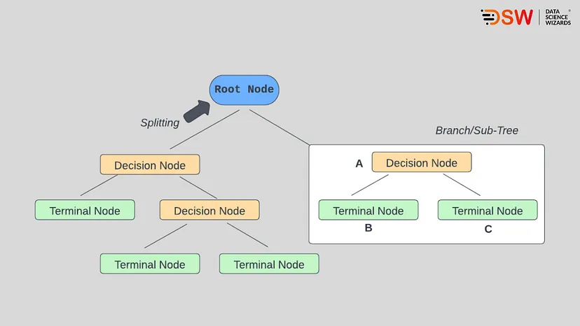
    decision-tree-algorithms

    Terminology

    Here, we need to understand the terminology we use with decision trees to understand the algorithm much better. However, it will also be the same for the random forest algorithms that can be thought of as extended versions of decision tree algorithms.

    Root nodes: as the name suggests, this is a node from which the decision tree starts. While looking from the data point of view, it is the point from which data populations start dividing according to various features.

    Decision nodes: As defined in the above picture, these are the node after the root nodes and are responsible for splitting the population into more nodes.

    Leaf nodes: These are the final nodes of the decision tree, after which further splitting of the data population stops.

    Sub-tree: Branches split from the root node can be considered the sub-tree from which the major population gets split.

    Pruning: This is a process of trimming some branches and nodes that we use to avoid overfitting.

    Here we have covered most of the terminologies we use with decision trees.

    First, let’s look at the example to know how this algorithm works.


    Example of Decision Tree

    Just take a look at the below data/table:
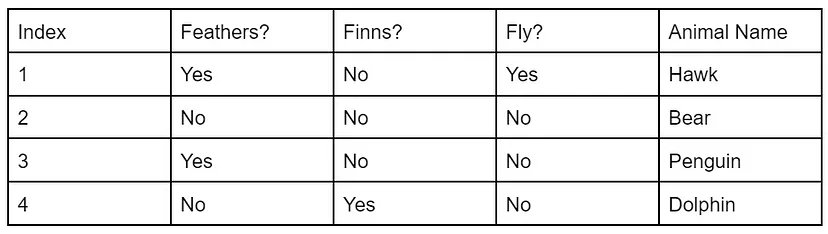
    example-of-decision-tree

    In the above data, we have information about feathers, Finns and flying status, using which we are required to tell the animal name. In such cases, the decision tree works in an upside-down nature, which means the root node(feather) will be on top, and the leaves(name of the animal) will be the last. For example, as given in the below image:
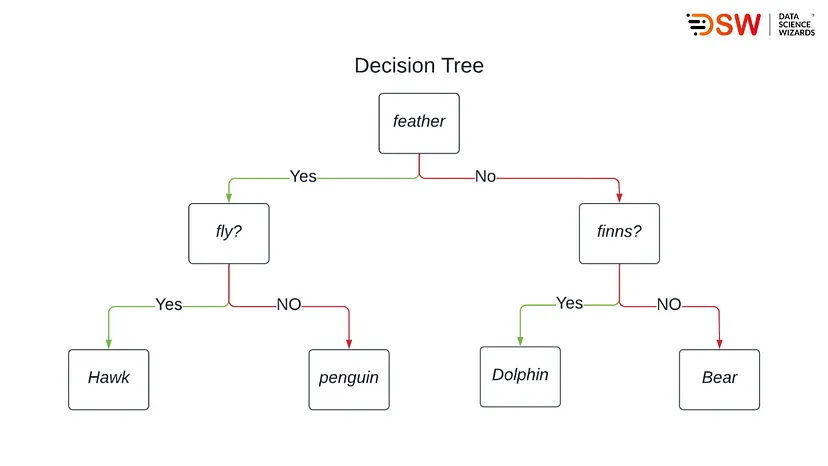
    decision-tree

    The above example is simple, but when we go deeper into the algorithms, we find that concepts like information gain, entropy and Gini index come before us. These concepts are beneficial in decreasing uncertainty or disorders from the model.

    For example, with large data sets, we may get confused about taking a feature as the root node and decision node, or we can also raise the question of where we should stop splitting. All uncertainty of modelling can be decreased by knowing these concepts. Let’s start with understanding entropy in decision trees.


    Entropy:

    In the above, we have seen that decision trees can be thought of as a bunch of if else statements and the confusion between if else becomes huge with large data sets. We can compare this confusion with uncertainty, and this uncertainty of the data s called entropy. We can also define entropy as the measure of disorder.

    Let’s look at an example of an object far from 9 viewers. The viewers are asked to identify the object, 4 out of 9 identify it as a table, and the other identifies the object as a bed. Because of this situation, it becomes difficult to tell what object is situated far, and this situation can be called randomness.

    The formula of entropy is as follows:

    entropy

    Where

    p+ = probability of positive class

    p– = probability of negative class

    S = Training example.

    Let’s see how entropy is used in decision trees.


    How is entropy used in decision trees?

    We can also compare entropy as a measure of impurity, and impurity is the degree of randomness. A situation can be called a pure sub-split if we get either yes or no.

    Let’s say in a feature, we have ten yes and five no in the root node, and after the first split, we have one decision node with six yes and four no. another decision node with three yes and two no.

    The above-given situation can not consider a pure sub-split because we have negative values in both decision nodes. So if we need to make a decision tree using such data, we are required to calculate the impurity of the split and once obtaining 100% purity, we can call the step a leaf node step or final step after which no split is required.

    To calculate the impurity, we use the formula of entropy.
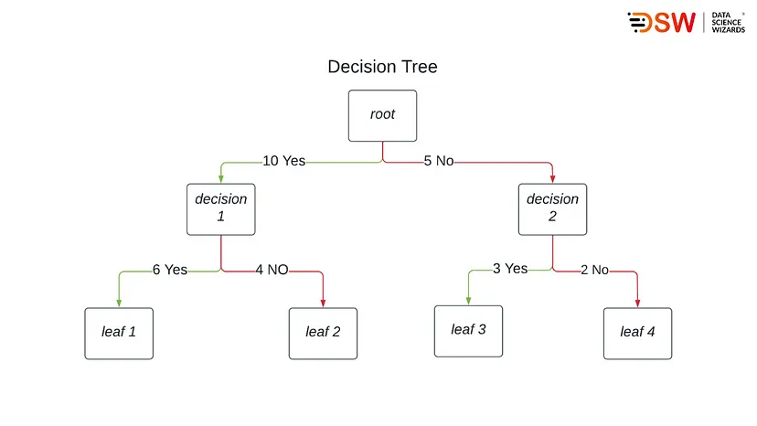
    entropy

    The above image tells us that our entropy for decision node 1 will be:

    E = -(6\10)log2(6/10) — (4\10)log2(4/10)

    E = -(0.6*-0.74) — (0.4*-1.32)

    E = 0.444 +0.528

    E = 0.972

    Entropy for decision node two will be:

    E = -(3\5)log2(3/5) — (2\5)log2(2/5)

    E = -(0.6*-0.74) — (0.4*-1.32)

    E = 0.444 +0.528

    E = 0.972

    In the above calculation, we can see that both nodes have the same entropy near one, and due to this, we can say that they also have similar low impurities because as the entropy increases, impurity decreases. Therefore, while deciding the entropy, we majorly focus on increasing the impurity.


    Gini Index

    When we talk about the Gini index, we find that somewhere its motive of work is similar to entropy. Both help finds the best feature for a split in the decision tree. The only difference between these two is the formula they use. The impurity of the feature after splitting the Gini index or Gini impurity can be calculated by the below formula:
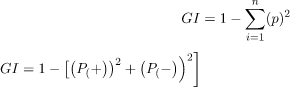
    Using this formula Gini index measures the impurity in randomly choosing an element, and it is preferable to use attributes with a lower Gini index or Gini impurity.

    Let’s take a look at the below data/table:
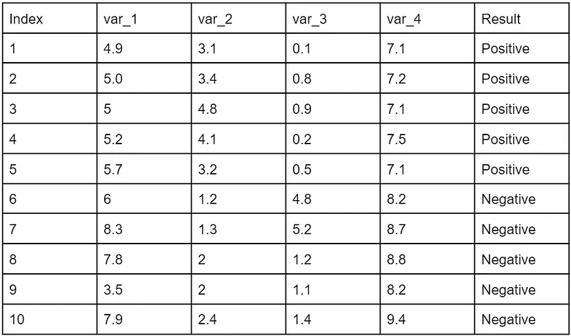
    gini-index

    In the above data, we can see that we have an equal proportion of negative and positive values. Using the Gini index, we randomly choose the values to categorise the attributes. Let’s say these values are as follows

    • Var_1: 6
    • Var_2: 2
    • Var_3: 2
    • Var_4: 9

    According to these values

    • If var_1 < = 6 then result = positive: 5/6
    • If var_1 <= 6 then result = negative: 2/6

    Gini(5,1) = 1- [(5/6)2 + (2/6)2 =0.19

    • If Var_1 > 6 then result = positive: 0/4
    • If Var_1 < 5 then result = negative: 4/4

    Gini(1,9) = 1- [(0/4 +(4/4)2] = 0

    Let’s calculate the Gini index using the above formula for var_1

    Gini(target,var-1) = 6/10*(0.19) + 4/10*0 = 0.096

    Similarly, the Gini index for other variables is as follows

    Gini(target,Var_2 = 0.375

    Gini(target,Var_3) = 0.375

    Gini(target,Var_4) = 0

    With these values we can design a decision tree as follows:
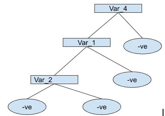
    gini-index

    In the above, we can see that we started splitting with variable 4, and as the Gini index increases, the population will get split accordingly.

    But this does not end because here, we get the entropy of a particular node. To get more splits, we must know about the parent node’s or child node’s impurity. Here information gain helps us in knowing about the parent node entropy. Let’s take a look at this concept.


    Information gain

    We mainly use information gain to measure the reduction of uncertainty when features are given. It also helps n deciding which attribute can be selected as the decision or root node.

    The formula for information gain is as follows.

    information-gain

    We can also think of it as entropy for the whole dataset. Let’s take an example of 60 people who are told to go and watch a movie and 32 out of 60 are going to watch the movie, and 28 of them are not.

    So to measure or predict this, we have two main features

    • Vehicle: yes or no
    • Class: below middle class, lower middle class and upper middle class.

    Using his two features, we can make our decision tree as follows.

    let’s calculate the entropy

    E(parent) = -(3260)log2(32/60) — (2860)log2(28/60) = 0.99

    E(parent|Vehicle = ‘High’ = -(2426)log2(24/26) — (226)log2(2/26) =0.39

    E(parent|Vehicle = ‘low’ = -(834)log2(8/34) — (26/34)log2(26/34) =0.79

    Let’s calculate the weighted entropy of each node:

    E(parent|Vehicle) =(26/60)*0.39+ (34/60)*0.79

    Accordingly, the information gained will be

    Information gain =E(parent) — E(parent|vehicle)

    Information gain = 0.99–0.62

    Information gain = 0.37

    In the above calculation, we can see that the parent entropy is near 1(0.99), which means if we take the vehicle as the root node, then the entropy of the dataset will decrease. If we follow similarly with the class feature, then using the below image:
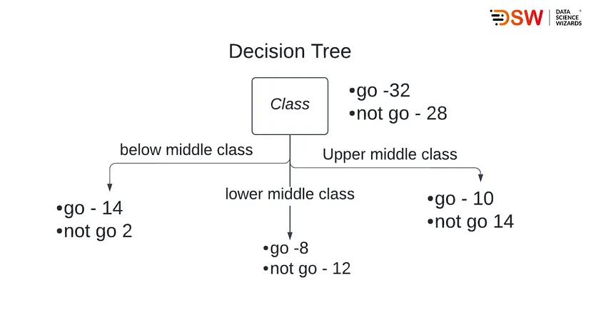
    decison-trees

    We can say,

    E(parent) = 0.99

    E(parent|Class = ‘below middle class’ = -(1416)log2(14/16) — (216)log2(2/16) =0.54

    E(parent|Class = ‘lower middle class’ = -(820)log2(8/20) — (12/20)log2(12/20) =0.97

    E(parent|Class = ‘Upper middle class’ = -(1024)log2(10/24) — (14/24)log2(14/24) =0.79

    Now let’s calculate the weighted average entropy of each node

    E(parent|class) = (16/30)*0.54 + (20/60)*0.97+(24/60)*0.98 = 0.86

    Here information gained will be

    Information gain =E(parent) — E(parent|Class)

    Information gain =0.99–0.86

    Information gain = 0.13

    Here we can see that reduction by class feature is 0.13 and the reduction by vehicle feature is 0.37. Hence we will select the vehicle feature to split nodes because it will have maximum information gain.

    According to the above process, if we select the vehicle feature for making root nodes, then we can say there are higher chances that people who have vehicles will go to watch the movie. After the root node, we can choose the class feature to split the population further.


    When to Stop Splitting?

    The most basic question raised by beginners that when to stop the growth of the decision trees. Before answering it, we need to understand that as the tree size increases, the chances of overfitting will also increase. Hence there should be an optimal length of a decision tree.

    In real-world problems, we are often required to deal with huge datasets that require a huge number of splits, and there are many ways to do that, like hyperparameter tuning, cross-validation, and gridsearchCV. In most of the modules used for building decision trees, we find the parameters max_depth, min_samples_split, min_sample_leaf and max_features. This parameter helps apply constraints over the decision tree after a pre-defined size tree reaches.


    Pruning

    It is also a way to avoid overfitting, especially for decision tree algorithms. In this procedure, we exclude some of the nodes and sub-nodes from the process. The non-significant nodes and sub-nodes can improve the chances of overfitting, and removing them can avoid overfitting and enhance the model’s accuracy. There are two main ways of pruning:

    1. Pre-pruning: This process cuts the trees when the trees are in the growing stages.
    2. Post-pruning: This process cuts the tree after it stops splitting. This is more significant than pre-pruning.

    Final words

    In this article, we have discussed a decision tree that follows very low mathematics behind still one of the reliable algorithms in the field of predictive analysis. However, since it differs from other algorithms, it has different terminologies. Moreover, it performs various actions on the data that split data and form a tree-like structure to reach the leaf node from the root node.

    In the following article, we will discuss the implementation of decision trees. To check our different articles, please refer to this link.
  • A Quick Guide to Deal with Missing Data

    A Quick Guide to Deal with Missing Data

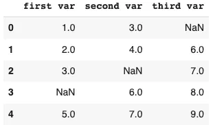
    In real-life data sets, we may find a considerable amount of missing value, sometimes these values can lead our data analysis and data modelling processes in the wrong direction. In general, we can define missing values as no record or datapoint stored for the variable in an observation or data gathering process. The below picture can be a representation of missing values:

    In the above image, NaN written on places is missing values. With the help of this Quick guide we learn the following things about missing values:

    • Types of missing values
    • Imputation techniques
    • Packages for imputations

    Let’s start by understanding the types of missing data.


    Types of missing values

    In general, there are three basic types of missing data.


    Missing completely at random(MCAR)

    As the name suggests, missed values are generated randomly in our data irrespective of relationships between any values, feature(observed or unobserved) and the missingness of the data.

    Examples:

    • Surveys where participants missed to fill any values.
    • Missed readings filled in any laboratory during any experiment.

    Missing at random(MAR)

    Values missed in a feature are not related to the feature itself but to other features in the data.

    Examples:

    • In any survey, women are less likely to give information about their age. It means the missing values are not related to the age feature but to the gender feature.
    • In any production line’s records, missing values generated for a component due to failure of different component comes under this category.

    However, MAR can become MACR when any condition or control is applied to the observed feature.


    Missing not at random(MNAR)

    if Values that are missed in a feature are related to the feature itself can be called MNAR. this type of missing value is most challenging to handle.

    Examples:

    • Participants are more likely to refuse to complete the survey about their unemployment.
    • In a survey, participants refused to talk about their pay scale.

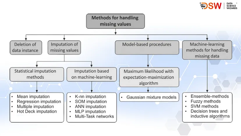
    Imputation techniques

    There are four main methods of handling missing data in datasets:

    • Delete missing values instance from data.
    • Imputation of missing data
    • Applying models like XGBoost that support the existence of missing data.
    • Use models for imputation of missing data like maximum likelihood estimation.

    Some standard replacement and mathematical methods to impute missing data.

    • Mean/Median imputation: Using this method, we can replace the missing values when the feature consists of continuous values.
    • K-nearest neighbour: this is a clustering process that tells about the nearest values, which can be used to fill missing values instances.
    • Multivariate Imputation by Chained Equations(MICE): in this method, we use machine learning models and different data features to predict the values for replacing missing values in a particular feature.
    • Iterative Regression Imputation: train a model for each feature with missing values.

    The below picture will let us know about these methods.

    handling-missing-values

    Packages for imputations

    There are various python packages to deal with missing values. Let’s take a look at these packages.


    Mean/Median/Mode imputation

    sklearn.impute.SimpleImputer(missing_values=np.nan, strategy=mean/meadian/mode’).fit_transform(incomplete_feature)

    Note: by just changing the strategy parameter, we can choose any method to impute missing values.


    k-nearest neighbours (kNN) imputation

    fancyimpute.KNN(k=n).fit_transform(incomplete_feature)

    Note: the k parameter is for a cluster number that needs to be defined as a numerical value.


    Matrix factorization (MF) imputation

    fancyimpute.MatrixFactorization().fit_transform(XY_incomplete)

    Multivariate imputation(Regularized Linear Regression)

    sklearn.impute.IterativeImputer().fit_transform(incomplete_feature)


    Multivariate imputation(Random Forest Regression)

    sklearn.impute.IterativeImputer(estimator= RandomForestRegressor().fit_transform(incomplete_feature)


    Final words

    In this quick guide, we have discussed small definitions of basic types of missing values that can harm our data modelling in real life. These missing values require different treatments that we discussed in the second section, and some python packages help in the treatment of missing values given in the third section.

  • End-to-End Logistic Regression Modelling

    End-to-End Logistic Regression Modelling

    In machine learning, Logistic regression algorithms are one of those basic models from which beginners start to learn classification modelling. Moreover, these algorithms are useful for modelling binary classification data. In one of our articles, we have already discussed how this algorithm work and how we should process it using synthetic data. In this article, we are going to use this algorithm with real-life datasets so that we can cover the following topics:

    • Data Exploration
    • Assumptions
    • Modelling
    1. Data processing
    2. Forward feature selection
    • Evaluation
    1. Confusion matrix
    2. Evaluation statistics
    3. ROC Curve
    4. Area Under the Curve

    Let’s start with gathering data. For this article, we will use a heart disease data set that shows us how different factors make a person diagnosed with heart disease. Let’s import this dataset in the form of pandas DataFrame.

    import warnings

    warnings.filterwarnings(‘ignore’)

    import pandas as pd

    data = pd.read_csv(‘https://raw.githubusercontent.com/TarekDib03/Analytics/master/Week3%20-%20Logistic%20Regression/Data/framingham.csv’)

    data.head()

    Output:

    regression-modelling

    Here we can see different factors that cause heart diseases. Some of them are categorical, and some of them are continuous data. Below, we can see the meanings of these variables:

    • Demographic variables:
    1. Male: Boolean or categorical data
    2. Age: Numerical and continuous data
    • Behavioural variables:
    1. Current smoker: Tell about current smoking habits(boolean)
    2. cigsPerDay: Average number of cigarettes consumed by a person in a day.
    • Medical(history):
    1. BPMeds: Whether a person consumes BP(blood pressure) medication(boolean)
    2. prevalentStroke: Previous stroke records(boolean)
    3. prevalentHyp: Prevalent hypertensive history(boolean)
    4. Diabetes: Diabetes status(boolean)
    5. totChol: Total cholesterol level (Continuous)
    6. sysBP: Systolic blood pressure (Continuous)
    7. diaBP: Diastolic blood pressure (Continuous)
    8. BMI: Body Mass Index (Continuous)
    9. heartRate: Heart rate (Continuous)
    10. glucose: Glucose level (Continuous)
    • Target variables
    1. TenYearCHD(ten year risk of coronary heart disease)(Boolean)

    In the above, we have seen that in the column male, we have values 0 and 1. Therefore, we are considering 1 as male and 0 as female and changing the data accordingly using the following lines of codes:

    data[‘male’] = data[‘male’].map({1: ‘male’, 0: ‘female’})

    data.rename(columns={‘male’:’Sex’},inplace = True)

    Lets perform basic EDA part on data before modelling it./


    Data Exploration

    Let’s begin with knowing the shape of data.

    print(‘shape of the data’, data.shape)

    Output:

    data-exploration

    In the data, we have 4240 data points and 16 variables, out of which 15 are independent, and 1 is dependent.

    Describing data

    data.describe()

    Output:

    data-exploration

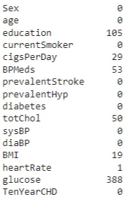
    Here we can see the data distribution, but it will be much better to see it using visualisation because the data size is large. Before the visualisation part, we should check for the null values.

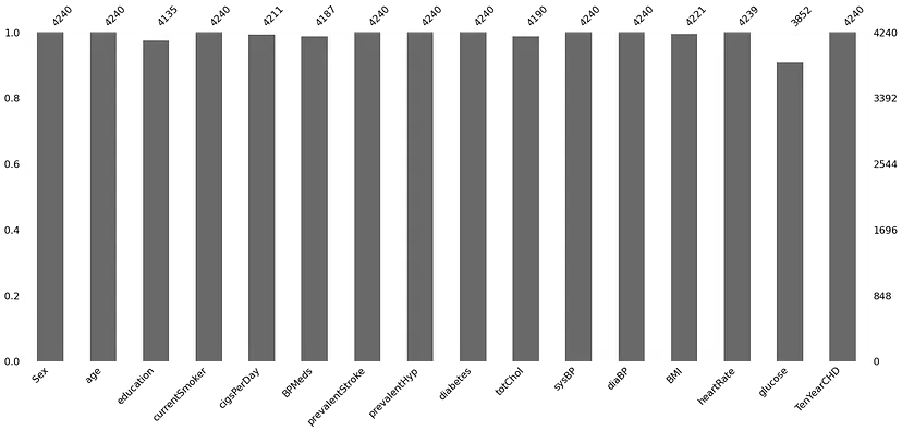
    import missingno as ms

    print(data.isna().sum(

    ms.bar(data)

    Output:

    data-explorations

    daat-explorations

    We can see that there are various null values present in multiple variables. Let’s see the total number of null values in the data.

    print(‘null values percentage’,round(data.isna().sum().sum()/len(data.index)*100

    Output:

    data-explorations

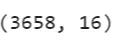
    We can see only 15% of values are null in the dataset, so instead of focusing on null values, we can delete them from the dataset.

    data.dropna(axis=0,inplace=True)

    data.shape

    Output:

    data-explorations

    Here we have completed the basic EDA of our dataset. Next, let’s understand data more using some visualisations.

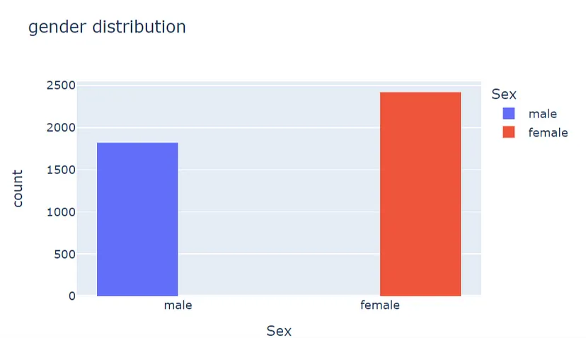
    Gender distribution

    import plotly.express as px

    fig = px.histogram(data, x=”Sex”, color=”Sex”,barmode=’group’,title = ‘gender distribution’,width = 600, height= 400)

    fig.show()

    gender-distribution

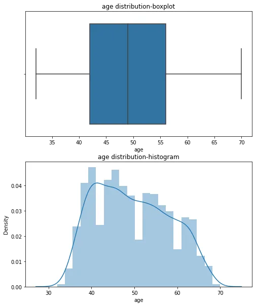
    Age distribution

    import matplotlib.pyplot as plt

    import seaborn as sns

    fig, axs = plt.subplots(nrows=2, figsize=(8, 10

    sns.boxplot(data[‘age’],ax=axs[0]).set(title=’age distribution-boxplot’)

    sns.distplot(data[‘age’],ax=axs[1]).set(title=’age distribution-histogram’)

    plt.show()

    Output:

    age-distribution

    In the above visualisation, we can see that most records are between the ages of 30 and 70, and the average age in the data is nearly 45 to 50.

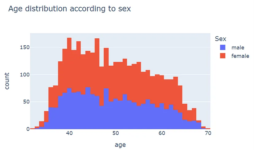
    Let’s see how the age variable is distributed according to gender.

    fig = px.histogram(data, x=”age”, color=”Sex”, title=’Age distribution according to sex’,nbins = 60,width = 600, height= 400)

    fig.show()

    age-distribution

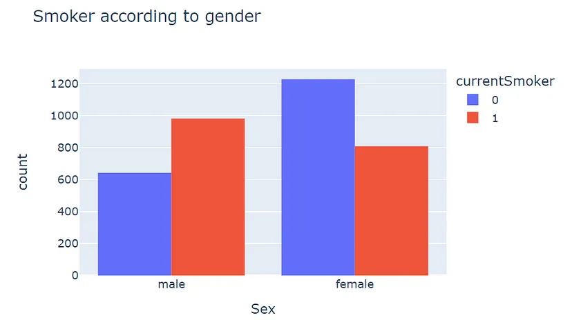
    This visualisation represents how the age of different gender is distributed, and by looking at it, we can say the distribution of females between 45 to 50 is higher than men. So now let’s see how many males and females are addicted to cigarettes.

    fig = px.histogram(data, x=”Sex”, color=”currentSmoker”,barmode=’group’,title = ‘Smoker according to gender’,width = 600, height= 400)

    fig.show()

    Output:

    smokers

    Here we can see that males are more addicted to cigarettes than the women. Now instead of plotting every feature from data we will try to merge them in one plot and try to understand how these features are related to each other.

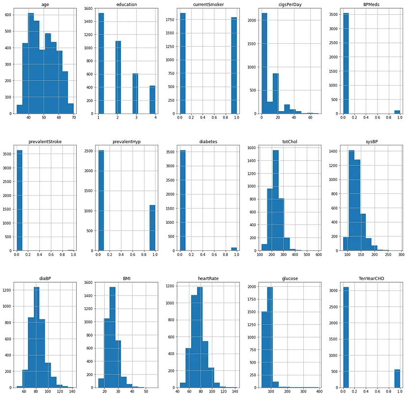
    fig, axis = plt.subplots(3,5,figsize=(20, 20

    data.hist(ax=axis)

    Output:

    output

    In the above, if we compare all plots with the plot of TenYearCHD, we can find that the graph of Bpmeds is similar to the TenyearCHD, which means if someone is taking medicines for blood pressure, then there are chances for that person to be on the risk of coronary heart disease.

    Also, the diabetes plot is similar to CHD and prevalentStroke, and prevalentHyp are pretty identical, and they can cause a significant effect on TenYearCHD.

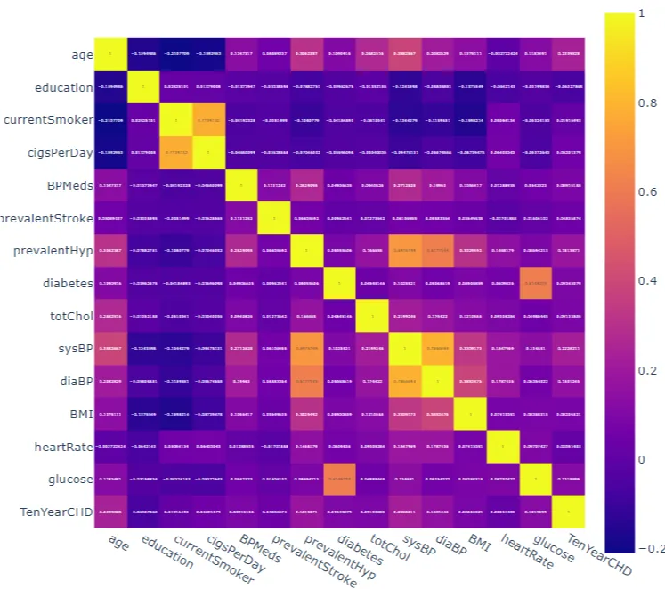
    Features with continuous data can explain themselves more using a correlation plot.

    corrmat = data.corr()

    fig = px.imshow(corrmat,text_auto=True,width = 700, height= 1000)

    fig.show()

    Output:

    ten-year-output

    Here we can see that various features are highly correlated to each other, and when we look at the plot, these values are positively correlated. Values like glucose level and diaBP always correlate to each other.

    Now here, our motive of data exploration is almost completed, and we should move toward the assumptions we consider in classification modelling.


    Assumptions

    In our last article, we have discussed five assumptions that we consider while using logistic regression for data modelling.

    1. Dependent variable with binary data points: In the above, we have already seen that TenYearCHD is binary data.
    2. Independent data points: Since collected data points are of different persons, there is no dependability between the data points.
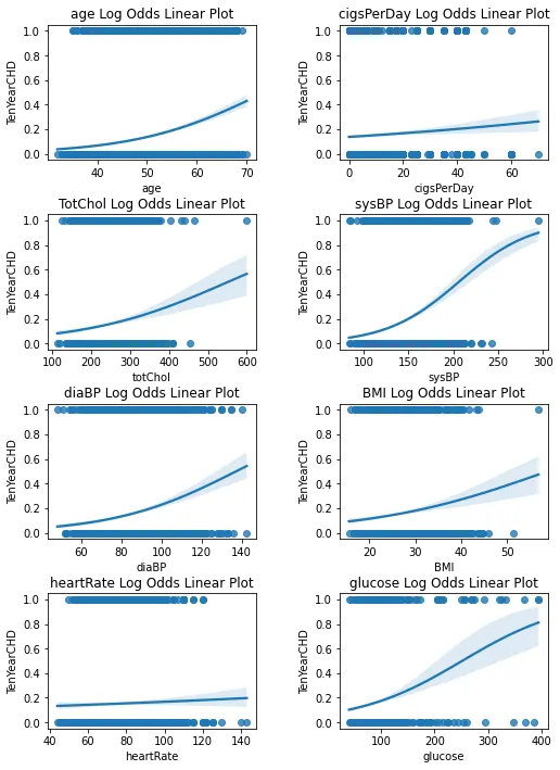
    3. Linearity between the independent variable and their odds: This assumption can be validated using a regression plot of the independent (continuous) variable. we can do that using the seaborn library:

    fig, axs = plt.subplots(ncols=2, nrows=4, figsize=(8, 10

    sns.regplot(x= ‘age’, y= ‘TenYearCHD’, data= data, ax=axs[0,0], logistic= True).set_title(“age Log Odds Linear Plot”)

    sns.regplot(x= ‘cigsPerDay’, y= ‘TenYearCHD’, data= data, ax=axs[0,1], logistic= True).set_title(“cigsPerDay Log Odds Linear Plot”)

    sns.regplot(x= ‘totChol’, y= ‘TenYearCHD’, data= data, ax=axs[1,0], logistic= True).set_title(“TotChol Log Odds Linear Plot”)

    sns.regplot(x= ‘sysBP’, y= ‘TenYearCHD’, data= data, ax=axs[1,1], logistic= True).set_title(“sysBP Log Odds Linear Plot”)

    sns.regplot(x= ‘diaBP’, y= ‘TenYearCHD’, data= data, ax=axs[2,0], logistic= True).set_title(“diaBP Log Odds Linear Plot”)

    sns.regplot(x= ‘BMI’, y= ‘TenYearCHD’, data= data, ax=axs[2,1], logistic= True).set_title(“BMI Log Odds Linear Plot”)

    sns.regplot(x= ‘heartRate’, y= ‘TenYearCHD’, data= data, ax=axs[3,0], logistic= True).set_title(“heartRate Log Odds Linear Plot”)

    sns.regplot(x= ‘glucose’, y= ‘TenYearCHD’, data= data, ax=axs[3,1], logistic= True).set_title(“glucose Log Odds Linear Plot”)

    # set the spacing between subplots

    plt.subplots_adjust(left=0.1,

    bottom=0.0,

    right=0.9,

    top=0.9,

    wspace=0.4,

    hspace=0.4)

    fig.show()

    Output:

    assumptions-output

    1. Here we are required to look at the shape of the plots. If plots resemble the s-shaped curve, we can assume that continuous independent variables are linearly related to their log odds. If any plot appears u-shaped, then we need to consider the data handling. In the above, every plot resembles the s-shaped or linear curve, so we don’t need to perform any data operation here.
    2. No Multicolinearity: No Multicollinearity: In the above, we have already seen a hugemulticollinearity between the independent continuous variable. We will deal With this multicollinearity later in the article.
    3. Enough data: Enough data: At the beginning of data exploration, we have seen more than 4000 data points available, which is quite enough to use logistic regression.

    Lets move toward the next section.


    Modelling

    In the above sections, we have explored data and looked at the assumptions we need to consider while modelling data using linear regression. In this article, we will use a technique called forward feature selection with a linear regression model to help us select the right features for modelling data using logistic regression. But before performing forward feature elimination, we are required to perform some of the data processing. So let’s start with data processing.


    Data preprocessing

    Converting the categorical values into numerical values

    data[‘Sex’] = data[‘Sex’].map({‘male’: 1, ‘female’: 0})

    Splitting the data into test and train sets.

    from sklearn.model_selection import train_test_split

    X = data.iloc[:,:-1]

    y = data.iloc[:, -1]

    X_train, X_test, y_train, y_test = train_test_split(X, y, test_size = 0.25, random_state = 42)

    Here we have converted 75% data into train and the rest of the data into the test. Now move towards the forward feature elimination process, and Before going into implementation, let’s understand this technique.


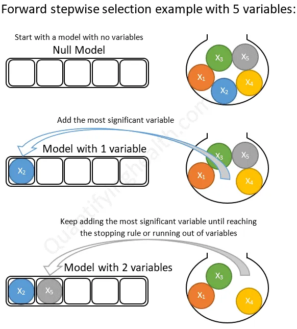
    Forward Feature Selection

    As the name suggests, it is a feature selection technique work iteratively. In the first iteration, it starts by putting zero features in the model and with each iteration, it keeps adding the rest of the features from the data. Finally, in the end, testing every feature throws the best model in front of us. The below image represents the forward feature elimination.

    feature-selection

    Image source

    Lets implement the forward feature elimination.

    sfs = SequentialFeatureSelector(LogisticRegression(n_jobs = -1),

    k_features = (1,14),

    forward= True,

    floating = False,

    verbose= 2,

    scoring= ‘accuracy’,

    cv = 5).fit(X_train, y_train)

    Output:

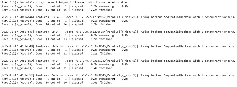
    fs-output

    Here in the above, we can see the history of the feature elimination process. And now, we can extract more pieces of information from this module, like the optimised feature used table of tests. Etc. Let’s check them.

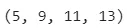
    Index of selected features

    sfs.k_feature_idx_

    Output:

    output

    Names of the selected features

    sfs.k_feature_names_

    Output:

    The Score of optimised model

    sfs.k_score_

    Output:

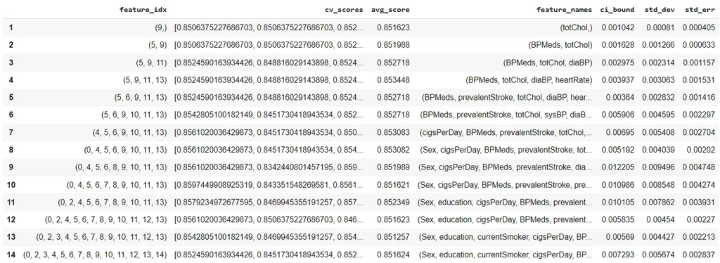
    Here we have chosen this method to perform because the data we have has multicollinearity, and we are required to extract features that can predict better. We can also look at the whole procedure of feature forward elimination.

    pd.DataFrame.from_dict(sfs.get_metric_dict(.T

    Output:

    Here we can see the accuracy of different models in the avg_score column. Let’s fit the logistic regression model with optimised features.

    Extracting the features from the main data

    new_features=data[[‘BPMeds’, ‘totChol’, ‘diaBP’, ‘heartRate’,’TenYearCHD’]]

    X=new_features.iloc[:,:-1]

    y=new_features.iloc[:,-1]

    X_train, X_test, y_train, y_test = train_test_split(X, y, test_size = 0.25, random_state = 42)

    Fitting the model and generating predictions based on the test set.

    lro=LogisticRegression()

    lro.fit(X_train,y_train)

    y_pred=lro.predict(X_test)

    After making predictions, we are required to evaluate the fitted model. the Logistic regression model can be evaluated in 4 methods. Let’s take a look at them.


    Evaluation

    Here we are going to evaluate our model using 4 methods:

    • Confusion matrix
    • Evaluation statistics
    • ROC curve (receiver operating characteristic curve)
    • AUC(area under the curve)

    Let’s start with our first methods.


    Confusion matrix

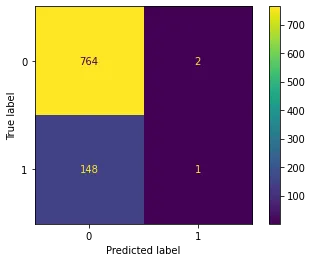
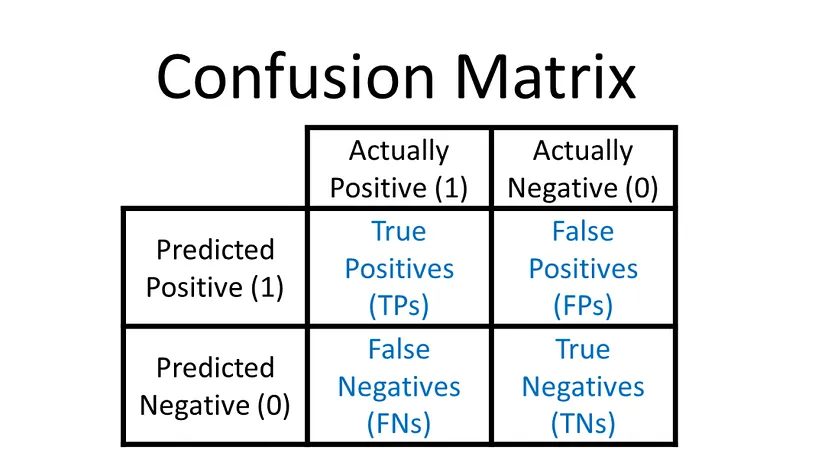
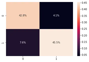
    this matrix will let us know how many right and wrong predictions the model generates.

    sklearn.metrics.plot_confusion_matrix(logreg, X_test, y_test)

    Output:

    confusion-matrix

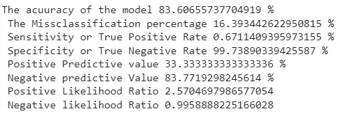
    Here we can see that (764 + 1) 765 values out of 915 are predicted right, and 150(148+2) are wrong. Based on the confusion matrix, we can evaluate our other evaluation statistics.


    Evaluation statistics

    TN=cm[0,0]

    TP=cm[1,1]

    FN=cm[1,0]

    FP=cm[0,1]

    sensitivity=TP/float(TP+FN)

    specificity=TN/float(TN+FP)

    print(‘The acuuracy of the model’,(TP+TN)*100/float(TP+TN+FP+FN),’% n’,

    ‘The Missclassification percentage’,100-TP+TN)*100/float(TP+TN+FP+FN,’% n’,

    ‘Sensitivity or True Positive Rate’,TP*100/float(TP+FN),’% n’,

    ‘Specificity or True Negative Rate’,TN*100/float(TN+FP),’% n’,

    ‘Positive Predictive value’,TP*100/float(TP+FP),’% n’,

    ‘Negative predictive Value’,TN*100/float(TN+FN),’% n’,

    ‘Positive Likelihood Ratio’,sensitivity/(1-specificity),’n’,

    ‘Negative likelihood Ratio’,(1-sensitivity)/specificity)

    Output:

    accuracy-ouptut

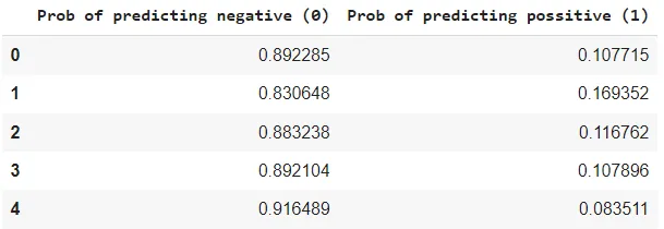
    Above are the evaluation statistics that tell us about the model’s accuracy, misclassification, positive and negative predicted percentage and other ratios. One thing I observed above is that model is more specific than sensitive. Also, it is more prone to calculate negative values correctly. So, let’s check the probabilities using which model is making predictions.

    pred_prob=logreg.predict_proba(X_test)[:,:]

    pred_prob_df=pd.DataFrame(data=pred_prob, columns=[‘Prob of predicting negative (0)’,’Prob of predicting possitive (1)’])

    pred_prob_df.head()

    Output:

    output

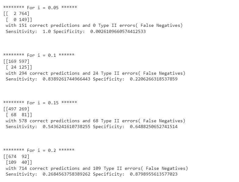
    In the above, threshold used by the model is 0.5(by default). Using this model should not be advisable because it is biased toward one class. We can iterate between other threshold values to make a better prediction.

    pred_proba_df = pd.DataFrame(logreg.predict_proba(X_test

    threshold_list = [0.05,0.1,0.15,0.2,0.25,0.3,0.35,0.4,0.45,0.5,0.55,0.6,0.65,.7,.75,.8,.85,.9,.95,.99]

    for i in threshold_list:

    print (‘n******** For i = {} ******’.format(i

    y_test_pred = pred_proba_df.applymap(lambda x: 1 if x>i else 0)

    test_accuracy = sklearn.metrics.accuracy_score(y_test.to_numpy().reshape(y_test.to_numpy().size,1),

    y_test_pred.iloc[:,1].to_numpy().reshape(y_test_pred.iloc[:,1].to_numpy().size,1

    print(‘Our testing accuracy is {}’.format(test_accuracy

    cm2 = sklearn.metrics.confusion_matrix(y_test.to_numpy().reshape(y_test.to_numpy().size,1),

    y_test_pred.iloc[:,1].to_numpy().reshape(y_test_pred.iloc[:,1].to_numpy().size,1

    print (‘With’,i/10,’threshold the Confusion Matrix is ‘,’n’,cm2,’n’,

    ‘with’,cm2[0,0]+cm2[1,1],’correct predictions and’,cm2[1,0],’Type II errors( False Negatives)’,’nn’,

    ‘Sensitivity: ‘,cm2[1,1]/(float(cm2[1,1]+cm2[1,0],’Specificity: ‘,cm2[0,0]/(float(cm2[0,0]+cm2[0,1],’nnn’)

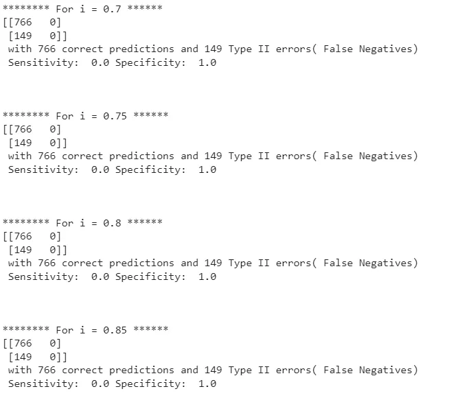
    Output:

    Part 1:

    part-1

    Part 2:

    part-2

    Here we can see that as the threshold gets lower, the model increases sensitivity, and after a threshold value, it is stable or decreases. So ROC curve can provide a more accurate picture.


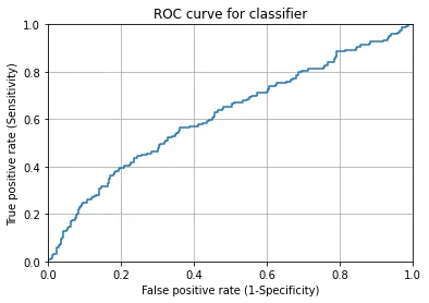
    ROC curve

    This curve lets us know about the performance of classification models when all classification thresholds are considered. On a fundamental note, it shows a trade-off between sensitivity and specificity of the model.

    y_pred2=logreg.predict_proba(X_test)

    fpr, tpr, thresholds = sklearn.metrics.roc_curve(y_test, y_pred2[:,1])

    plt.plot(fpr,tpr)

    plt.xlim([0.0, 1.0])

    plt.ylim([0.0, 1.0])

    plt.title(‘ROC curve for classifier’)

    plt.xlabel(‘False positive rate (1-Specificity)’)

    plt.ylabel(‘True positive rate (Sensitivity)’)

    plt.grid(True)

    Output:

    roc-curve

    Looking at the above, we can say that the optimum position for the ROC curve is at the top left corner because a model can be a good classifier only if it can predict more true positives than False positives. Let’s check the area under the curve.


    Area Under the Curve(AUC)

    The area under the curve can be considered representative of the model’s accuracy because the higher area shows us a higher disparity between the true and false positive and higher capability of the model to classify training data. However, a good measure of AUC starts from 0.5, and as it goes towards 1 it represents better classification.

    print(‘Area Under The Curve(AUC): ‘,sklearn.metrics.roc_auc_score(y_test,y_pred2[:,1]

    Output:

    Looking at the AUC, we can say our model is a moderate classifier.


    Final words

    In the above, we have seen how we can perform classification modelling using logistic regression modelling. During the process, we look at the data insights. After that, we used forward feature elimination to choose the right features from the data to get higher accuracy in modelling. We have also gone through Some of the assumptions we need to take care of during modelling and some of the evaluation techniques we can use to evaluate the model correctly. In the end, we can make following colclusion:

    • Forward feature elimination helped find significant features that can impact heart disease prediction.
    • Data analysis told us men are more addicted to cigarettes and susceptible to heart diseases.
    • Total cholesterol is an important predictor of heart disease.
    • The model we made is more specific than sensitive.
    • AUC is around 0.62, which is quite satisfactory.
    • The model requires more data from category one, so the class imbalance problem can be sorted.

    References

    link to the codes

  • Why are data scientists using Feature Stores?

    Why are data scientists using Feature Stores?

    When we look at the data science field, we see many different technologies are gaining momentum because they are making data modelling easier, more flexible and more accessible. Feature store is one of those technologies and becoming the need of data scientists. This technology is used in the field to maintain the flow of data between database and model. Since it is very helpful in improving the way and performance of modelling we should be aware of it. In this blog post, we are going to talk about the feature store using the following points.


    Table of content

    • What is a Feature?
    • What is a Feature Store?
    • Why Feature Store is beneficial for Data Scientists?
    • Why UnifyAI’s Feature Store?

    What is a Feature?

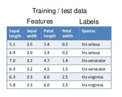
    The reader should know that machine learning models work based on past information. In most examples, we find that data is in tabular form where rows are data points, and columns are attributes describing those data points. A feature is an attribute that we use to describe each example.

    In a simple modelling procedure, we use mathematical algorithms that help make predictions based on the old examples for the new examples. This process is called inference. The old example generally refers to training data and feature engineering is a process where the modeller applies transformation and selection to raw data so that suitable features can be consumed by the model.

    feature

    In the above example of data, we can see that there are four features and one target variable in the iris data.


    What is a Feature Store?

    A feature store can be thought of as a tool storing features that are useful for the ML model, and when it comes to training or prediction time, it serves the old or new data to the model.

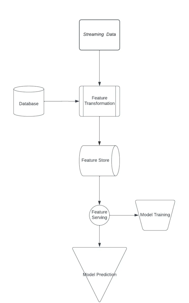
    After looking at the above points we can infer that A feature store is a start point of the modelling procedure and end point of data flow because this is where a data scientist easily access and discovers data to train, evaluate and execute machine learning models.

    It takes place in the system because it helps in keeping track of the lifecycle of the data which the model is using. We can consider it as a junction where we group the features created in the multiple data sources. Purposely feature stores are being utilised to ensure data correctness, maintain the data flow, and reuse the features.

    In case of adding new examples, the feature facilitates previously developed features pre-computed so that the availability of features for inference can be maintained.

    feature

    The above flow chart explains the place of feature stores in the modelling procedure.

    Why feature store?


    Why Feature Store is beneficial for Data Scientists?

    Feature store is not an old technology that comes in front of us. Instead, the first public feature store was applied by Uber in 2017 named Michelangelo Palette. Feature store helps in solving some of the major data modelling problems:

    • Exclude higher complexities during development

    In the above points, it is discussed that the modelling procedure consumes data in two places, one in training and the other in inference. Talking about the training time, we find that data consumption happens in batches and old databases and BigData options provide the facility of serving data in batches.

    When it comes to inference time, it is suggested not to rely on a batch prediction strategy. If the feature store and batch prediction strategy are not there, then data scientists require to set up different solutions for each new project.

    • Exclude complexities in debugging models in production

    A good feature store applied in modelling provides a facility to retrain and debug the model when in production it is not performing as expected. This facility is called point-in-time correction and becomes very helpful in retraining and checking the model with the same data and new data.

    • Cost reduction in feature reusability

    When applying ML models in an organisation, it is found that there are always more than one use-cases that need to be resolved using the same feature from the data. If feature store is not applied, reusing the similar feature for a different use case requires a new set-up and costly storage. Feature stores provide flexibility of reusing the feature for different use cases.

    • Reduces the effect of feature drift

    This one is the most important point in favour of the feature store. When new examples come into the databases, the data distribution changes and this causes the degradation of the model, which is not trained with a new example. Feature store provides the facility of retraining the model on new data. This feature of the feature store helps in maintaining the model performance.


    Why UnifyAI’s Feature Store?

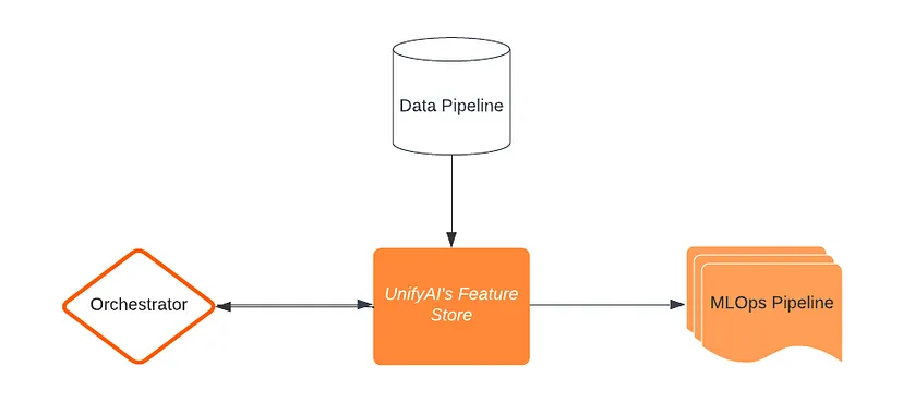
    We at DSW are democratising the power of AI using our flagship platform UnifyAI. This platform uses some essential components to build, orchestrate and leverage AI capabilities for use cases across the domains, and the feature store is one of those components. Using feature store, this platform helps reduce the time of building and resolving new use cases. Understanding and working with feature stores is easy but understanding its placing in an end-to-end development procedure is complex. A feature store always requires a place from which it can take part in model building as well as in model orchestration. Using the full capability of feature stores, UnifyAI ensures we can resolve use-cases as much as possible using common features. This reusability of features from the feature store helps us reduce time into processes like data validation, cleaning and transformations. This time reduction helps UnifyAI focus more on model accuracy and performance. Other components connected to feature stores are:

    • Data Pipeline: gives features to feature stores
    • MLOps Pipeline: Extracts features from feature stores.
    • Orchestrator: Fetch required features

    The below diagram tells the basic story of UnifyAI’s feature store.

    data-pipeline

    Also, In the above sections, we have seen how feature store plays an important role in the data science process. We understand and keep ourselves up-to-date with such useful and new technologies and take responsibility for utilising them with real-world problems wit the aim of making AI work for everyone.


    Final Words

    As many organisations from every domain are thinking of applying AI and ML to resolve their use cases, it becomes essential to understand how they can utilise their data fruitfully. Moreover, as technology is gaining momentum, it becomes compulsory to understand the trending topics in the technology field and topics that are beneficial in opting. Feature store is one of those techniques which not only improves the quality of AI-enabled decisions but also scales the capacity of taking AI-enabled decisions.


    About DSW

    Data Science Wizards (DSW) is an Artificial Intelligence and Data Science start-up that primarily offers platforms, solutions, and services for making use of data as a strategy through AI and data analytics solutions and consulting services to help enterprises in data-driven decisions.

    DSW’s flagship platform UnifyAI is an end-to-end AI-enabled platform for enterprise customers to build, deploy, manage, and publish their AI models. UnifyAI helps you to build your business use case by leveraging AI capabilities and improving analytics outcomes.

    Connect us at contact@datasciencewizards.ai and visit us at wordpress.datasciencewizards.ai/

  • The landscape of Data Engineering in 2022

    The landscape of Data Engineering in 2022

    Year by year, enrichment of the field by a variety of products has been witnessed, and still, the development is following an exponential graph. Every year our data engineers and data scientists are required to get hands-on with different technologies and tools. This article will inform us about the data engineering landscape in 2022. Let’s start with our first section.


    Data Ingestion

    The primary motive behind data ingestion is to obtain some data and process it toward storage or immediate use. We can say that data ingestion is taking ourselves inside or absorbing something out of data.

    In the real world, this is a layer consisting of streaming technologies and SaaS services that connect pipelines between operational and data storage systems.

    Recently, we found a significant rise in Airbyte that is helping to get a custom ETL data pipeline running in very little time. Airbyte was founded in 2020, and the short period they have taken to get more than 15,000 organisations are its user, and there are more than 600 contributors to it.

    Facilitating the market with reverse ETL that we consider very different from the ETL, the motive behind reverse ETL is to put the data into operational systems, and the process becomes beneficial to the workflow of the system and organisation.


    Data lakes

    Data lakes are subjected to holding the object under them. Between 2019 and 2020, we have seen an enhancement in the complexity for data engineers to keep critical structure data and analytics engines together.

    The enhancement of complexity made it a compulsion for us to separate data lakes and analytics engines. So in essential points, organisations are storing objects in data lakes and producing different databases to optimise and analyse the data.

    Such methods of data engineering and analytics have different reasons for being introduced in the industry. One of the common reasons is a cost consideration. As the size of data is increasing cost of analysing data in data lakes like snowflake and BigQuery also increases. So instead of analysing the data in data lakes, managing usable data in a small storage system becomes cheaper on both computation and cost basis.

    Although famous data lakes, Databricks and Snowflake include data lakes and analytics engines, we can still consider your optimised version of Spark SQL as an analytics engine to analyse the most sable data in Delta Table format. With Snowflake, we can find support for Iceberg as external tables to its database.


    Metadata analytics

    A simple explanation of metadata can be “data of the data”, which explains the characteristics of data like a summary does with a book.

    In current scenarios, organisations are more focused on descriptive and organisational metadata. Being competitive in the field, organisations are spending more and more time evolving their storage and computer facilities so that they can become supportable for the scale of data.

    In recent days we can observe major problems that organisations face are with the analysis and management of metadata.

    One of the most efficient ways to store data in data lakes is advancing regularly. Some of the significant projects like Delta from Databricks, Onehouse by Apache Hudi, and Apache iceberg by Tabular are making substantial changes in the industry being open-source projects.

    Since Large commercial entities are applying these projects and making it difficult for other projects to influence the market through their facilities. Being open-source and projects of the apache/Linux foundation provide a low risk to the community.

    Examples such as Hive Metastore are being replaced with open table formats because not all of them are capable of utilising the metadata and metadata storage properly. While looking at the git for data, we can say that somehow it is keeping its position in continuity.

    Git for data is making engineers utilise the practices of versioning which don’t support the maintenance and management of metadata in data lakes. On the other hand growth of DataOps is also continuous that making organisations control and manage dataset versioning while containing similar data over time. The LakeFS, Census, Mozart Data, and Databricks Lakehouse Platform are one of those options for opting DataOps, which helps with data versioning and keeping itself growing in the industry.


    Data computation engine

    This section talks about how the data is getting distributed throughout the organisations and different processes. We can spread this section into two categories distributed computation engine and data analytics engine. The significant difference between these categories lets us know how the platforms are opinionated with storing data into different layers.

    • Distributed compute engine: Instead of being concerned about the storage strategies of data These engines are the SQL codes that help engineers to distribute data and are majorly concerned about the programming language. Using these data can be stored in many formats and sources. Ray and Dask are the perfect examples of such an engine that are very new and based on the popular Python programming language. Spark is maintaining itself as the ruler of distributed engine scenario.
    • Data analytics engine: These engines are concerned with data storage capacities and computational costs. A variety of competitors in this category are there, like Snowflake, BigQuery, Redshift, and Firebolt. Examples of some old-school warehouses are PostgreSQL and Databricks lakehouse. However, they all are concerned with the data formatting and performance of the querying engine.

    Orchestration

    Like always, Airflow is leading this market as an open-source product with the support of Astronomers. The acquisition of Datakin made Astronomers more strong because now it has the capability of providing data lineage.

    They claim that by utilising this feature, organisations can make a safer and more resilient pipeline than before. The Data lineage tool helps understand the nature of data and performs analysis using traditional ways without any outer interventions.


    Data analytics and ML usability

    It is simply a place where pipelined data is going to be used for making insights from the data and modelling the data using machine learning algorithms. We can also say that this place is the final place for the data going to be modelled because afterwards, MLOps is going to manage the data.


    Machine Learning Operations (MLOps)

    MLOps are a set of practices that take a model from modelling to production. However, under these operations, we use various tools that are good enough to perform a certain task but lack when they are expected to provide other aspects of the ML pipeline. Still, provision end-to-end ML solutions are available, and in 2022 tools and companies like Comet, Weights & Biases, Clear.ml and Iguazio are emerging.

    Some other new tools are also available, like Activeloop and Graviti. These are newer age tools and developed appropriately. Able to understand the complexity of data, management of data and complex data operations.

    dagsHub is one of those approaches which can provide an E2E problem solution as an open-source platform. This can also be a solid approach to getting an end-to-end solution.


    Model quality management

    Under the MLOps processes, we need tools to manage the quality of models throughout the production process. Day by day, these tools are growing rapidly, and Deepchheck is one of the results of this growth. As a result, many contributors, partners and traction can be witnessed for this tool.


    Catalogues, permissions and governance

    Any size company is understanding and working on the space of data catalogue. It becomes a compulsion across the competitors in the market. Some companies like Alation and Collibra are still expanding themselves by including more offerings than before.

    BigID is also trying to enhance itself by providing catalogue offers. Immuta is also persistent in offering data access control services while utilising newer technologies to become compatible with additional data sources.


    Final words

    This year, we have observed that the landscape of data engineering is rapidly growing in every aspect. Furthermore, many contributors are helping this landscape to grow while growing themselves. As a result, a massive amount of change and innovations can be seen in the field that is impacting the area immensely.

    As the dimensions to go of the data are expanding, the rush of different open-source technologies towards the development in every data field can be observed. Data engineering is an excellent example of this rapidly growing field where technologies such as MLOps, DataOps, and Metadata analytics have recently added and expanded to a great level.


    About DSW | Data Science Wizards

    Data Science Wizards (DSW) is an Artificial Intelligence and Data Science start-up that primarily offers platforms, solutions, and services for making use of data as a strategy through AI and data analytics solutions and consulting services to help enterprises in data-driven decisions.

    DSW’s flagship platform UnifyAI is an end-to-end AI-enabled platform for enterprise customers to build, deploy, manage, and publish their AI models. UnifyAI helps you to build your business use case by leveraging AI capabilities and improving analytics outcomes.

    Connect us at contact@datasciencewizards.ai and visit us at wordpress.datasciencewizards.ai/

  • Introduction to No Language Left Behind (NLLB-200)

    Introduction to No Language Left Behind (NLLB-200)

    Meta AI recently open-sourced its massive translation model, No Language Left Behind (NLLB-200), intending to exclude language barriers across the globe. As we know, that machine translation has become a key area of research nowadays, and it has become a great news for many researchers and organisations who can use it for their respective research and work. So let’s take a look at the news and understand a bit about NLLB-200 with the below points:


    Table of contents

    • What is NLLB-200?
    • Advancement in NLLB-200
    • Where is NLLB-200 applied?
    • The training procedure for NLLB-200

    What is NLLB-200?

    No Language Left Behind (NLLB-200) is a model from the series of massive machine translation models of MetaAI for language translation. A newer member of the series NLLB-200 is capable of translating between 200 languages, representing Meta’s capacity of Meta in the direction of AI researchers. These development aims to allow people to access, share and use online content in their native languages and communicate across the world regardless of language preferences.


    Advancement in NLLB-200

    Some of the significant advancements in this model are:

    • According to the Meta AI research team, this model can provide 44% better results than the previous versions.
    • This model is also capable of translating languages Kamba and Lao. These languages were not translated before using any of the machine translation methods available freely.
    • To train this model, they have generated a new dataset named Flores-200 consisting of data in 200 languages.
    • Evaluation of this model has gone through 40,000 different translation directions.
    • It can translate content from one language to another without using any intermediate language, for example, directly from Hindi to Thai.

    Where is NLLB-200 applied?

    Meta AI is utilising this project on their platform on Facebook and Instagram to enhance communication in various languages. These platforms are highly responsible for connecting people together. According to an article on statista there are roughly 2.93 billion active users of Facebook in the first quarter of 2022. Looking at these statistics, we can understand how useful this model is for not only Facebook but also for the people using Facebook because they become more effective when using their native languages.

    The technology behind this project is also available with the Wikimedia Foundation’s Content Translation tool, which helps Wikipedia to translate the content into different languages. This is very beneficial for the world because it will produce more knowledge in more languages.


    The training procedure for NLLB-200

    These three major steps involved in the training procedure of NLLB-200:

    1. Automatic data construction: To make this model work on low-resource languages, Meta used the teacher-student training procedure where the older LASER(Language-Agnostic SEntence Representation) model is trained on 200 languages and produced a huge amount of data for training of NLLB-200.
    2. Modelling 200 languages: A large number of expert models has been utilised in the modelling so that every category of the data or language can be routed under the shared capacity settings of models. In addition, regularisation techniques are utilised to avoid overfitting of the models. This step can be compared with the normal machine translation modelling procedure where one encoder and one decoder are utilised first to translate word data into numerical form and then again into the word form.
    3. Result Evaluation: For evaluation of the results from NLLB-200, meta has extended their dataset FLORES to cover 200 languages. The dataset consists of human-translated data. Utilising various metrics and human evaluation support, they have validated that the model is producing 44% better results than Meta’s older machine translation models.

    Final words

    In this article, we have gone through big news in the field of machine translation modelling. NLLB-200 is one of the major changes because it’s being utilised for translation between 200 languages. In advancement, we can see the major directions where this field is extending itself. This technology has helped advance some of the major platforms that are required to deal with considerable language barriers. Training procedures of these models can help in understanding the procedure of modelling big algorithms. We can learn more about this open-source model here.

    References

  • Introduction to EDA

    Introduction to EDA

    In every field where data plays a crucial role, whether it is data analysis, engineering, or modelling, data analysis and investigation, we can say data exploration becomes one of the major tasks to perform before going forward with the data. Therefore, to start your journey in the field of data science, it is always suggested to start by knowing exploratory data analysis(EDA). In this article, we will discuss the exploratory data analysis (EDA) using the following points:


    Table of content

    • What is Exploratory Data Analysis(EDA)?
    • Why is EDA important?
    • Types of EDA
    • Steps involved in EDA
    • Exploratory Data Analysis tools

    What is Exploratory Data Analysis(EDA)?

    Before working with data, we must understand that data’s characteristics. The exploratory data analysis can explain features/characteristics of the data and understanding of the data. EDA is a process that helps people to understand data, discover patterns of data, and perform hypothesis testing from the data.

    EDA plays a crucial role in making a business decision based on old data records. EDA can represent the data using different charts that can be interpreted as a summarisation of the tabular data. EDA also involve mathematics expressions such as standard deviations, categorical variables, and confidence intervals.


    Why is EDA important?

    EDA becomes essential for any business and allows data analysts, engineers and scientists to analyse and understand data just before consuming it in any process. Mainly EDA ensures that the results after the processing are applicable and valid to business outcomes and goals.

    Some other points that make EDA important include:

    • It helps in identifying errors in data
    • It helps in detecting outliers or anomalous data points and events.
    • It helps in drawing and understanding the relationship between variables.
    • Visualisation makes decision-making easy.
    • It helps in understanding background processes.

    Types of EDA

    There is mainly four types of EDA we find:

    1. Univariate non-graphical: One of the simplest forms of EDA or data analysis used to understand the data and patterns of the data. This type of analysis includes only one variable of the data, which is the reason it is not capable of telling the cause and relationship.

    2. Univariate graphical: This can be considered an advanced form of non-graphical EDA which is capable of giving more insight from the data than the non-graphical EDA. common Univariate graphical EDA includes:

    • Stem-and-leaf plots, help in representing the distribution of the data.
    • Histogram, helps in representing the frequency or proportion of classes for a range of values.
    • Box plots, help in representing the summary of data in terms of minimum, first quartile, median, third quartile, and maximum value of data.

    3. Multivariate nongraphical: When more than one variable is available, this kind of EDA helps in representing the relationship between those variables utilising cross-tabulation or statistics.

    4. Multivariate graphical: This kind of EDA uses visual graphs from the data with more than one variable to represent the relationship between variables. Grouped bar charts with each group representing one level of one of the variables can be a typical example of Multivariate graphical EDA.

    Some other common examples of this type of EDA include:

    • Scatter plot, Helps in representing the relationship between two variables by drawing data points in two-dimensional or three-dimensional space.
    • Multivariate chart, Helps in representing the relationship between factors and response.
    • Heatmap, Helps in representing the correlations between variables using the density of colours.

    Steps involved in EDA

    Some of the basic steps of an EDA process include:

    1. Data collection: the first step start the EDA is to have data from the data source and analyse it at a higher level. It just includes the following things:

    Determining the size

    Data points observation

    Description of dataset

    2. Missing value optimisation: this step requires finding the missing value under the data set. After finding it, we are required to recognise the source of the missing value and how we can handle such values by just deleting or filling them.

    3. Data categorisation: This step includes the categorisation of the data values so that it can become helpful in performing statistical analysis and visualisation of the data. Following main categories, a dataset can include:

    Categorical

    Continuous

    Discrete

    4. Relationship Identification: this step helps in finding the relationship between data variables. For example, the category of weather can be optimised using values of humidity, pressure and wind speed. This example tells us about how weather can change because of continuous values. Finding correlations helps in deriving independent and dependent variables.

    5. Outlier detection: after finding the correlation, one step that makes the data processing more accurate is outlier detection. There is always a possibility of the existence of such values in the data, which is different from the other data points. These values become very harmful in data modelling. So it is always suggested to perform this step to avoid wrong data modelling safely.


    Exploratory Data Analysis tools

    Python and R are the most common tools for EDA:

    • Python — It is an object-oriented programing language which includes a lot of libraries like Pandas, Numpy, Matplotlib, Seaborn and Scipy, which makes it one of the best tools to use for data analysis. Pandas library is beneficial for data analysis. Matplotli, Seaborn and Plotly are some libraries that help visualise data. Being easier in terms of coding also makes this language a widely used language for data analysis and data modelling.
    • R — it is an open source programming language that gives various facilities to perform statistical computations and analysis, including multiple aspects of data visualisation. This is also a widely used programming language amongst data scientists, analysts and engineers.
    • SPSS: SPSS is one of the main tools/software to utilise for statistical analysis. This software has been developed to perform statistical analysis in social science. Although this can be utilised for performing EDA for every kind of data and supports the interactive user interface, it differs from Python and R programming languages.

    Conclusion

    In this article, we have discussed the EDA, which helps data analysts, engineers and scientists to understand the data by finding essential patterns and information hidden inside the data. Along with this, we have also talked about its importance and steps that can be included while performing EDA. Python and R tools are primarily used tools for performing EDA and can be a good point for beginners to start with EDA.


    About DSW

    Data Science Wizards (DSW) is an Artificial Intelligence and Data Science start-up that primarily offers platforms, solutions, and services for making use of data as a strategy through AI and data analytics solutions and consulting services to help enterprises in data-driven decisions.

    DSW’s flagship platform UnifyAI is an end-to-end AI-enabled platform for enterprise customers to build, deploy, manage, and publish their AI models. UnifyAI helps you to build your business use case by leveraging AI capabilities and improving analytics outcomes.

    Connect us at contact@datasciencewizards.ai and visit us at wordpress.datasciencewizards.ai/

  • BLOOM- A new member in the NLP space

    BLOOM- A new member in the NLP space

    On the 12th of July 2022, the world of artificial intelligence and data science (specifically NLP) got exciting news in the Large Language Models(LLMs) field. The BigScience, an open collaboration of Hugging Face, GENCI and IDRIS and one of the most extensive research workshops in the field of NLP, has introduced complete transparency and open sourced multilingual large language model BLOOM clipped form of BigScience Large Open-science Open-access Multilingual Language Model. Let’s talk a bit more in detail using the following pointers.


    Table of content

    • What is BLOOM?
    • Who can use BLOOM?
    • Technical specifications

    What is BLOOM?

    Bloom is one of those autoregressive large language models capable of generating text from a prompt on a massive amount of text data. This model is not limited to one language; it can produce such text in 46 languages and 13 programming languages. Furthermore, this model can also be extended to perform such NLP or text tasks it has been explicitly trained for, just by casting the process as a text generation task.

    It is the first complete transparent multilingual LLM that took 176 billion parameters and the Jean Zay supercomputer for training. Building this model required the engagement of 1000 researchers from 70+ countries and more than 250 institutions for 117 days of training.


    Who can use BLOOM?

    Any one individual or organisation wanting to try and investigate this model can download, run and study from here. Before utilising it, we require to agree to these terms and conditions.

    Since it is embedded in the Hugging Face platform, its implementations are the same as the other transformers of Hugging Face. This means it can be imported with transformers and run with accelerates.

    This model can be utilised in some real-world use cases that require text generation like writing recipes, information extraction from articles, or composing new sentences utilising the series of texts. Also, it is an excellent example for many aspirant data science developers and researchers from where they can start their journey of learning software like PyTorch, apex, DeepSpeed etc., in a deeper direction.


    Technical specification

    BLOOM is a modified version of Megatron-LM GPT2 that includes only decoder architecture. Talking about the parameters and layer space, it contains 176 billion parameters, 70 layers and 112 attention heads with 14336-dimensional hidden layers. The objective function enabled by the model is cross entropy with mean reduction.

    As discussed above, this model got trained on Jean Zay Public Supercomputer, which was provided by the French government. Some of the specifications of this computer are as follows:

    • 384 A100 80GB GPUs (48 nodes)
    • CPU: AMD
    • CPU memory: 512GB per node
    • GPU memory: 640GB per node
    • Inter-node connect: Omni-Path Architecture (OPA)

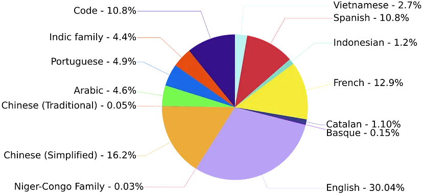
    Training of this model took 1.6TB of text(pre-processed), and the below pie chart represents the text distribution according to language in training data.

    bloom

    The model’s training started on the 11th of march, and it is estimated that the end date of the training is 5th July 2022. The number of Epochs utilised in training is one, and the estimated cost of the training is Equivalent to $2–5M in cloud computing.

    There are the following versions of BLOOM is available:

    • bloom-350m
    • bloom-760m
    • bloom-1b3
    • bloom-2b5
    • bloom-6b3
    • bloom (175B parameters)

    Final words

    We have seen what it takes to build this model and how it can help the Data Science community. By looking at the various things, we can say that it has the potential to become revolutionary in the field of NLP as the development team is considering it as just a beginning and not just a one-and-done model. You can try the BLOOM model here.


    About DSW

    Data Science Wizards (DSW) is an Artificial Intelligence and Data Science start-up that primarily offers platforms, solutions, and services for making use of data as a strategy through AI and data analytics solutions and consulting services to help enterprises in data-driven decisions.

    DSW’s flagship platform UnifyAI is an end-to-end AI-enabled platform for enterprise customers to build, deploy, manage, and publish their AI models. UnifyAI helps you to build your business use case by leveraging AI capabilities and improving analytics outcomes.

    Connect us at contact@datasciencewizards.ai and visit us at wordpress.datasciencewizards.ai/

  • How is Artificial Intelligence Advancing Banking Domain?

    How is Artificial Intelligence Advancing Banking Domain?

    In recent years, we can witness that artificial intelligence is becoming a need in every domain of the industry, and AI’s different domains, such as computer vision, natural language processing, and predictive modelling, are helping humans solve their use cases and problems more effectively and without the intervention of the humans. We can also enjoy the intervention of AI in our daily life, and humans are becoming more curious about this intervention. Banking sectors are also positively affected by the intervention of AI. In this article, we will cover some of the critical use cases of AI in the banking sector that is helping humans advance the banking sector.


    Customer Engagement

    banking-domain

    This sector implies AI-enabled models to assist the customer during onboarding. These models are trained to perform step-by-step processes of customer onboarding. Natural conversation utilises digital channels. Bots are there to automate the services like processing the documents of customers and taking images from computer vision programs.

    Some other vast implementations of OCR systems can be found to process the documents of the customer, and a variety of systems are there that help in performing document verifications of customers to make the customer onboarding faster and smooth. Since no human intervention is required, fewer human skills are necessary. It also helps the service provider to prevent their human workforce from performing repetitive and sometimes mundane tasks inside the premises.

    WeChat messenger is an excellent example of engaging customers by utilising conversations. For instance, China Merchant Bank is one of the largest credit card companies using WeChat messenger to handle 1.5 to 2 million customers.


    Customer Service

    customer-service

    In a banking system, customer care, service and engagement programs play a crucial role in democratising the bank’s services among the customers and also help in enhancing sales and marketing of banking services. Nowadays, it is found that chatbots have replaced humans in customer care, and this also impacted the banking sector. While applying chatbots in such systems delivers a very high ROI in cost savings.

    Embedding chatbots in the banking sector can be considered the most common application of AI in the banking sector. There are various tasks such as balance inquiry, statement production, and fund transfer that can be managed using these chatbots and applying such chatbots helps in reducing the overload of the channels like contact centres and internet banking channels.

    HDFC bank’s chatbot named EVA is an excellent example of this use case where we can consider it as the banking assistance for the customers of HDFC and helping them with things like Branch addresses, IFSC codes, loan and interest rate information.


    Automatic Advice Systems

    automatic-advice

    In traditional banking and finance systems, we find that banks employ humans to advise the customers and clients regarding investments, loaning, credit cards and debit card schemes. However, as the number of customers and their requirements increases, it becomes challenging for humans to manage such big data and provide beneficial advice to everyone.

    Artificial intelligence and data science intervention in banking and finance systems have made this task very easy. AI-enabled models are being developed and prepared to perform automatic advice procedures with a touch of personalisation for everyone. These models are learned to give the best advice to customers according to the requirements, and that makes them a personalised advice system in banking. Also, they are beneficial in reducing the time of the banking procedures.

    For example, ICICI banks in India blended an RPA( robotic process automation) with their systems and successfully cut loan processing time in half.


    Predictive Analysis and Modelling

    predictive-analysis

    One of the most common use cases of artificial intelligence is to perform predictive analysis and modelling using the data. These modelling procedures find the correlation between the data points and variables and tell about the future possibilities. Traditionally it was complicated to understand and predict such possibilities, and the intervention of AI models made it very easy. Using such models, we can have information about sales opportunities, cross-sell opportunities, share market statistics and social media channels. These pieces of information can lead to a direct revenue impact. We can also calculate metrics around operational data in the banking system so that predicting values can become an easy task. There are various examples of static models and neural networks being consumed frequently to predict near or far future trends and patterns.


    Security

    security

    AI can be utilised for security purposes, which not only helps in the banking system but also allows being applied in different domains. For example, we know that models work by understanding patterns hidden in the data, so if data about the previous threats are given to these models, they can help us find current and future threats. Furthermore, these predictions can help baking systems to prevent attacks and fraudulent activities.

    There is various software such as SEON, SAS, ThreatMetrix and Feedzai that is helping in preventing banks from threats and fraud. For example, Citi bank employs Feedzai for three significant protections: securing account openings, controlling transaction fraud, and stopping money laundering.

    Security on the premises of banks is also the main topic to be covered when it comes to security. These security purposes include enabling security cameras and security guards throughout the premises. Artificial intelligence also helps these systems to enhance the level of security by utilising face recognition and biometric systems. However, these systems can also be integrated with bank applications to enhance the security on the customer side.


    Credit Scoring

    credit-scoring

    One of the major impacts of AI on the banking system can be found in credit scoring, where the model trained using the history and demographics of users can help determine the creditworthiness of clients and customers. Such an application becomes very helpful for the banking systems where they can predict the credit scores in a very robust and accurate way.

    Since demographics are applied in training, these models sometimes don’t require a vast history of the users and can work by comparing the demographics of the other users to tell the credit score of a new user.

    Softwares such as GiniMachine, LenddoEFL, ZestFinance, Kreditech and SAS Credit Scoring are leading AI-enabled software for credit scoring.


    Decision Making

    decision-making

    Various decisions can be taken using historical data, which can have a high impact on the banking systems. Such models work in a system where expert data is stored in a database and utilised to make strategic decisions like deciding workflow between different departments, cash flow management, and document flow strategy within the bank.

    Various banks are utilising analytical AI-based tools such as AlphaSense, which is an AI-enabled search engine that uses the processes of Natural Language Processing and also helps with task routing.

    Conclusion

    In the banking sector, the intervention of artificial intelligence has put a lot of scope in various tasks in the knowledge workforce and in preventing banks from cyber risks and fraudulent activities. Enabling AI in banking sectors has enhanced the competition between different banks. AI models are improving banking services from being applied to customer services to making impactful strategic decisions.


    About DSW

    Data Science Wizards (DSW) is an Artificial Intelligence and Data Science start-up that primarily offers platforms, solutions, and services for making use of data as a strategy through AI and data analytics solutions and consulting services to help enterprises in data-driven decisions.

    DSW’s flagship platform UnifyAI is an end-to-end AI-enabled platform for enterprise customers to build, deploy, manage, and publish their AI models. UnifyAI helps you to build your business use case by leveraging AI capabilities and improving analytics outcomes.

    Connect us at contact@datasciencewizards.ai and visit us at wordpress.datasciencewizards.ai/

  • Getting Started with Machine Learning Algorithms: Logistic Regression

    Getting Started with Machine Learning Algorithms: Logistic Regression

    In the field of data science, we mainly find a variety of algorithms or models to perform regression and classification modelling. Logistic regression can be considered the first point of your learning line of data science, classification and predictive modelling. Since it comes under the regression model family it uses a curve to classify data in classes. We at DSW highly prefer to model small use-cases and problems utilising such small algorithms because these are highly robust and easy to interpret. In this article, we are going to talk about logistic regression. Let’s just start by what the logistic regression algorithm is.


    What is logistic regression?

    Logistic regression is one of the most basic and traditional algorithms or models that comes under the supervised machine learning classes used for classification and predictive modelling. In basics, these algorithms can be used to model the probability of an event or a class. Since it comes from the regression class models it uses the lines or curves to model the data and we use it where the dataset we have can be separated using lines, and the outcome from the model is required to be binary or dichotomous.

    That means we use logistic regression for binary classification and binary classification works when the target variable is separated into two classes. Simple examples of binary classification are yes/no, 0/1, win/loss etc.

    There are two types of logistic regression

    • Simple logistic regression
    • Multiple logistic regression

    Where simple logistic regression is utilised where only one independent variable is affecting the dependent variable and multiple logistic regression is utilised when there are more than two independent variables affecting the dependent or target variable.

    However, this can also be extended to the multinomial logistic regression and ordinal logistic regression where the number of classes is discrete in more than two classes or more than two classes of an ordinal nature. Since we majorly believe that using one line we can not separate more than two classes accurately we are going to learn about the simplest versions of logistic regression that can be utilised for binary classification. Let’s see how this algorithm works.


    How does Logistic Regression Work?

    As discussed above logistic regression works by separating linear separable data just like linear regression. To understand the working of logistic regression we are required to understand the mathematics behind it.


    Mathematics

    Let’s consider there is one predictor or independent variable ‘X’ and one dependent variable y and the probability of y being 1 is P. In such a situation the equation of linear regression can be written as:

    p = mx + m0 …..(1).

    The right side of the above equation is a linear equation and can hold beyond the range 0 to 1. And we all know that probability can vary between 0 to 1 only. So to overcome that we can predict odds in place of probability using the following formula:

    Odds = p/(1-p)

    Where,

    p = probability of occurrence of any event.

    1-p = probability of non-occurrence of any event.

    According to odds, 1 can be written as:

    p/(1-p) = mx + m0 .….(2)

    Here we also need only a positive number that can be handled using the log form of the left side of equation 2.

    log(p/(1-p)) = mx + m0 …..(3)

    To recover the above equation we need to use the exponential form of both side

    e(log(p/(1-p)) = e(mx + mo) …..(4)

    While simplifying equation four we will get the following equation

    p = (1-p)(e(mx + mo)) ..…(5)

    We can also write this equation as follows

    p = p((e(mx + mo))/p — e(mx + mo))

    p =e(mx + mo)/(1 + e(mx + mo)) .….(6)

    Now we can also multiply e(mx + mo) / e(mx + mo) on equation 6.

    p = 1/(1 + e-(mx + mo))

    Above is the final probability that logistic regression uses if the above-given condition is true. But if there are n predictors then the calculatory equation will be as follows

    p = 1/(1+ e-(m0+m1x1+m2x2+m3x3+ — — +mnxn))

    The above is the final equation of logistic regression when there is n predictors. Some experienced persons compare this equation with the sigmoid function because it also controls the range of output between 0 to 1.

    In the above, we can see how we started with the linear equation and ended with the curve.

    A Mathematically sigmoid function can be written as follows:

    (z) = 1/(1+e-z)

    In the above, we are required to replace z with e-(mx + mo) to make it an equation of logistic regression. Looking at the equation we can say the below image will be a representation of the working of logistic regression.

    mathematics

    In the above image, we can see how logistic regression keeps the curve between the values 0 and 1. Now before utilising logistic regression on any data we are required to consider some of the assumptions. Let’s take a look at the assumptions.


    Assumptions

    Before modelling data using a basic logistic regression algorithm we are required to consider the following assumptions:

    • If any extensions are not applied then data needs to have a dependent variable with binary data points.
    • The data points under the data need to be independent of each other.
    • The independent variables of the data need to have no or small multicollinearity with each other.
    • The independent variables and their odds need to be linear to each other.
    • One thing that sometimes becomes mandatory according to the suggestions is that it is good to work with a large data size while utilising logistic regression in the process.

    Here we have seen some of the assumptions that need to be covered before applying logistic regression. Let’s see how we can apply logistic regression to any data.


    Implementation

    In this section, we will look at how we can apply logistic regression to data using the Python programming language. However, we can also use R, MATLAB and excel for performing logistic regression but considering the size of the article we are using only Python.

    In Python, Sklearn is a library which provides functions for applying every kind of machine learning algorithm in our datasets and for applying logistic regression we have the LogisticRegression method under the linear_model package which we utilise here.

    Let’s start with making a synthetic dataset using the make_classification function of Sklearn.

    from sklearn.datasets import make_classification

    X, y = make_classification(n_samples=1000, n_features=5, random_state=42)

    Here we have created a dataset which has 1000 rows and 5 columns in the independent variable dataset and 1 dependent variable with two classes 0 and 1. We can validate it by converting these arrays in the pandas DataFrame.

    import pandas as pd

    df = pd.DataFrame(data=X)

    df[‘Target’] = y

    df

    Output:

    output

    Here we can see all the independent and dependent variables in one place.

    Before going for modelling we are required to know which variables from our dataset have a better correlation with the target variable. Let’s check the correlation.

    import seaborn as sns

    corr=df.corr()

    sns.heatmap(corr, annot=True,

    fmt=’.1%’)

    Output:

    output

    Here we can see that variables 0, 1, and 3 have higher correlations with the target variable and we can consider them in the data modelling with logistic regression.

    Let’s trim and split the datasets

    X = X[:, [0,1,3]]

    from sklearn.model_selection import train_test_split

    X_train, X_test, y_train, y_test = train_test_split(X, y, test_size = 0.29, random_state = 0)

    Let’s import the function from Sklearn and model the data.

    from sklearn.linear_model import LogisticRegression

    model = LogisticRegression()

    model.fit(X_train, y_train)

    Let’s make some predictions so that we can validate the model

    y_pred = model.predict(X_test)

    y_pred

    Output:

    array-output

    Here we can see the prediction made by the model. Now we need to evaluate this model.


    Evaluation

    Evaluation of a classification model can be done in various ways. Since it’s a binary classification model we find that there are two prime methods which can help us in the evaluation. These methods are as follows:


    Accuracy score

    It is the universal method for evaluation of any classification model which mainly compares actual and predicted values using the following formula

    accuracy(y,ŷ) =( 1/nsample)i=0nsample-11(ŷ=yi)

    Where,

    y = actual values

    ŷ= predicted values

    This simply calculates error predictions and gives the calculated error in the form of percentage values. Let’s see how we can calculate it for the above model.

    from sklearn.metrics import accuracy_score

    print (“Accuracy of binary classification : “, accuracy_score(y_test, y_pred)*100,”%”)

    Output:

    accuracy

    Here we can see the accuracy of our model is good enough. Let’s verify it using another evaluation method.


    Confusion matrix

    This method tells us how many right decisions were taken by the model. As the name suggests this is a matrix which holds the following values under the cells

    confusion-matrix

    Here we can see that the true positives and true negatives are the values that the model has predicted right and other values are wrongly predicted. Let’s check how many right values our model is predicting right from the test data.

    import seaborn as sns

    cm = confusion_matrix(y_test, y_pred)

    sns.heatmap(cm/np.sum(cm), annot=True,

    fmt=’.1%’)

    Output:

    output
    accuracy

    In the above, we can see that 11.7% (7.6 + 4.1) values are not accurately predicted by the model and 88.3% values are correctly predicted. Let’s take a look at how the logistic regression model is being utilised in the real world.


    Application of logistic regression

    There are a variety of use-cases that can be found solved using logistic regression in a variety of fields like medical, politics, engineering and marketing. For a simple example, these models can be utilised to predict the risk of disease development in a human body by observing its characteristics or for predicting the mortality of injured humans and animals.

    In politics, we can use it for predicting the number of voters in an election who are going to vote for a party by observing the demographics of voters. In engineering, we find that this model is being utilised for the failure optimization or prediction of various components, processes and systems. In marketing, it is being utilised for predicting the propensity of customers regarding the purchase of any product or service using the analysis of demographics of customers.

    This model can be extended to perform operations in different domains of AI where sequential data is being collected and analysed like NLP and computer vision.


    Final words

    In this article, we have discussed one of the basic algorithms in machine learning which is logistic regression. There are a variety of use cases where we can find this algorithm most reliable. For instance, it has been utilised for predicting the mortality of injured humans in Trauma and Injury Severity Score (TRISS). Such examples make us believe that for some simple cases we can rely on logistic regression.

    References


    About DSW

    Data Science Wizards (DSW) is an Artificial Intelligence and Data Science start-up that primarily offers platforms, solutions, and services for making use of data as a strategy through AI and data analytics solutions and consulting services to help enterprises in data-driven decisions.

    DSW’s flagship platform UnifyAI is an end-to-end AI-enabled platform for enterprise customers to build, deploy, manage, and publish their AI models. UnifyAI helps you to build your business use case by leveraging AI capabilities and improving analytics outcomes.

    Connect us at contact@datasciencewizards.ai and visit us at wordpress.datasciencewizards.ai/